Okay, I posted this Excel Chart Challenge on Friday. How did you do? I am sure your solution is better than mine. This was the challenge from an Excel Forum question:
“How to eliminate outliers in graph
When viewing some graphs, sometimes I need to ignore some outliers. Like to know whether it is possible to click on the outlier data or the corresponding x on the x axis and the graph will be updated without this outlier data. I know I can go to the data set and remove the outliers but want to simplify by doing it on the graph. Many thanks.“
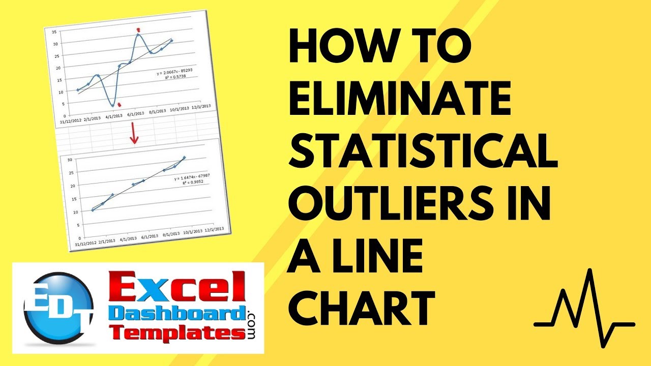
Here is the picture that this user posted:
The graph has 2 outlying data points. 1 on January 4th and 1 on January 7th. The Excel user manually deleted the data points and then you will see the final chart on the bottom of the picture.
We need to also add a trendline with a trend line formula and R value but this can be a manual step. The data goes from January 1st to January 10th in the year of 2013. So lets go with these assumptions.
So how can we create the final chart by removing the data points from January 4th and January 7th without manually deleting those data points? Lets get to it! Below you will find a quick breakdown on how I created my solution. Below that is a detailed step-by-step tutorial of this Excel solution. Below that you will see a Video demonstration of this Excel tip. Finally, below that you will find a copy of my spreadsheet that you can download to plan around with the data and charting technique.
First off, let me show you how another user tackled this problem. Pete had an ingenious way around this problem. He takes the data points and creates a formula based on the slope of the line. Here is his solution in his own words:
From Pete: “I was playing around with your new Friday challenge, and I came up with a different spin on the results. My chart shows the original data, and the new data with the outlyers removed. You will have to unlock the sheet to view the formulas.
Basically, I took the original data and used the SLOPE function to find the slope of the data, and then compared it to a theoretical line based on the X value using the algebraic formula for lines Y=MX+B. With this formula and the calculated slope, I could solve for B. Now I used and IF formula to return a #N/A error if the real value and theoretical value differed by a given % chosen by the data validation drop down cell. This way the user can choose at what percent at which to remove the outlyers. I had to include 500% and 100% to allow the user to show the original data as the data point “2” is 710% away from the calculated theoretical value.“
Check out his solution here: Petes Outlyer Solution
Now here is my basic solution for creating an Excel Line that doesn’t display Outliers. Come back tomorrow to see my advanced solution.
The Breakdown
1) Create Chart Data Range
2) Designate a Cell as the Outlier Tolerance Level
3) Create Outlier Formula for Chart Data Range
4) Create Outlier Chart in Excel
5) Add Trendline to Chart, Trendline Formula and R-Squared Value
6) Smooth the line and clean up Chart Junk
Step-by-Step
1) Create Chart Data Range
Okay, lets create our original data range in cells A1:B11. Now lets create a quick line chart in Excel with markers to see what it looks like. Looks almost exactly like the first chart that you saw from the original question. 
Only difference is that our line is not smoothed. The last step in this tutorial will show you how to make this change. But here is what the original chart would look like with Smoothed Lines:

2) Designate a Cell as the Outlier Tolerance Level
Okay, my solution uses a spreadsheet cell to designate what the tolerance is for an outlier. So I have designated cell D3 in the spreadsheet as my tolerance level. Looking at the data, it appears that a data point is designated as an outlier in the Excel user’s example when the points differ about 7 units.
So I have put in a value of 7 in cell D3:
We will use cell D3 in the next step when we create our outlier formula.
3) Create Outlier Formula for Chart Data Range
First, lets put our dates in cell E2. This is as simple as putting an =A2 in cell E2.
Okay, this is the step that makes everything work. What we need to do is compare the current data point with the data points above and below the current one. The comparison will see if the current data point is outside of the tolerance level we set in cell D3. Essentially, we are going to subtract the current data point from the data point one cell above and see if the difference is greater than the tolerance in cell D3. Then repeat this step for the cell below the current data point. If both data points are greater than the tolerance level, then we will put a NA() in the current cell. If both values are not out of tolerance, then we will put the value of the current data point in this cell. Now because the difference could be negative, we need to wrap this subtraction in an absolute value function. So in cell F2 let’s put this formula:
=IF(AND(ABS(B2-B1)>$D$3,ABS(B2-B3)>$D$3),NA(),B2)

Here is a breakdown of the formula:
First we are going to start with an IF formula, so go to cell F2 and type this:
=IF(
because we need to compare a value and then based on that value we will put one of 2 values in this cell
Now as I described above, you need to compare the current data point with the cell above and the cell below. And, if both comparisons are out of tolerance, then we don’t want to show the data point. So, since we are dealing with a “BOTH” comparison, we should use the AND function, so lets type that in next:
=IF(AND(
Now as I stated earlier, sometimes subtracting the data points will make the final value Negative. And a negative value will ALWAYS be below our tolerance, so we need to make sure that our difference is always in positive units since our tolerance level is in positive units. To make something always positive, we need to wrap our comparison in an Absolute Value function, so let us type in the ABS function next:
=IF(AND(ABS(
Now lets actually make our 1st comparison value. We do this simply by subtracting the current value with the value above the current data point and see if it is greater than our tolerance level in cell D3. So type that in:
=IF(AND(ABS(B2-B1)>$D$3
Note that I made the D3 and absolute reference. If you don’t know what an Absolute Reference is, check out this post:
Referring to Ranges in Formulas for your Excel Dashboard Templates
That is the first part of our AND function and the and function is separated by a comma then you will put the next comparison. So lets type in the next comparison after a comma. The next comparison is to compare our current data point with the next data point. So lets type that in:
=IF(AND(ABS(B2-B1)>$D$3,ABS(B2-B3)>$D$3
Since that is our last comparison that we need to worry about, you can end the AND function with a right parenthesis. Now we can put a comma in and determine what to do if both of the AND criteria are true. In our case, if both the differences of the data points are greater than the tolerance, then we need to put a NA() function in there. So lets type in that IF TRUE value:
=IF(AND(ABS(B2-B1)>$D$3,ABS(B2-B3)>$D$3),NA()
If you want to learn more about the NA() function, check out this post:
How-to Hide a Zero Pie Chart Slice or Stacked Column Chart Section
Now we are ready for the final value if the AND function is NOT TRUE. So put a comma in and type in the IF FALSE value. In this case, we want to put in the actual data point value of our data cell B2. So type in a comma and then B2)
=IF(AND(ABS(B2-B1)>$D$3,ABS(B2-B3)>$D$3),NA(),B2)
Now press enter and your value in Cell F2 should look like this:
Now that we have our formulas in place, we can copy them down to our last data point in columns A and B. So copy this formula down and it will look like this:
Notice that data points for 1/4 and 1/7 are now showing a value of #N/A. And the other values are the same as you see in our original data set in Column B. That is SO WONDERFUL! What a cool excel tip to get rid of outliers from our trend.
Now we are all set to build our Excel outlier chart.
4) Create Outlier Chart in Excel
So lets create our chart by highlighting the cell range from E1:F11. Then go to the Insert Ribbon and select a Line Chart with Markers from the Line button:
Your chart should now look like this:
It looks a lot different then the one with the outliers:
5) Add Trendline to Chart, Trendline Formula and R-Squared Value
Now that we have our chart, we just need a few last things. Let us add a trendline to our chart. To do this, click on the chart and then click on the chart line. From there, go to the Layout Ribbon and choose the Trendline button and then choose Linear Trendline:
Then choose “Linear” and “Display Equation on chart” and “Display R-squared value on chart” from the Format Trendline dialog box: 
Your chart will now look like this:
6) Smooth the line and clean up Chart Junk
Now all we need to do is clean up the chart and we are all set! First select your chart and then select the legend and press your delete key. Your chart should now look like this:
Now we need to create a smoothed line chart. To do that, select the chart and then the line in the chart. From there, press your CTRL+1 key to bring up the Format Series dialog box. From there, select the LIne Styles from the left menu and choose Smoothed Line from the Line Style choices:
Your final chart should now look like this:
Not much difference, but when your data has greater changes, it will look even more smooth ![]() .
.
Now lets compare it to the original request. It looks almost exactly like what we wanted. However, you will see that the data points from January 3 to the 5th is joined and not broken like the original sample. Sam for data points between 1/6 and 1/8. I am not sure how critical it is to NOT have these lines connect, but it is not possible with the way Excel creates line charts when you have a gap of data that uses a formula.
However, come back tomorrow where I will show you how to make a line chart show a gap using formulas.
Video Tutorial
Check out this video demonstration of building an Excel Line Chart that Ignores Outliers:
File Download
You can download my free Excel Line Outlier Chart Template here:
How-to-eliminate-outliers-in-an-Excel-graph-basic-method.xls
Also, don’t forget to sign up as a subscriber! And please try and share this site with your Excel co-workers and friends. It is much appreciated.
Steve=True


