I recently had a request from a fan of the site on how they could make a dynamic pie chart with the Top 5 values. The user had to create this pie chart regularly from a larger data set and wanted to know how they could do this easily.
The user thought that they would need to use a combination of Index and Match or some other formula to find the Top 5 values and was concerned if there were ties and how it might change if there were less than 5 top values.
Well there is an easy solution for this and Excel had done the heavy lifting for us. The other great thing is that this technique will also work for many other chart types like Column and Bar charts in Excel.
So lets show you how you can do this in just a few short steps.
The Breakdown
1) Create Pivot Table
2) Set Pivot Table Filter for Top or Bottom Values
3) Create Pivot Chart
4) Refresh Pivot Table Data
Step-by-Step
1) Create Pivot Table
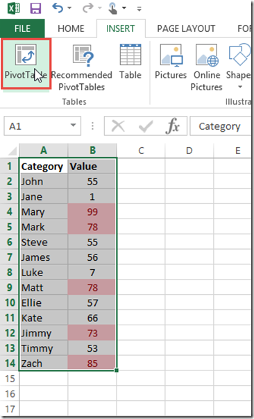
First we need to create a Pivot Table. You can do this by highlighting your data set and then click on the Insert Ribbon and then click on the Pivot Table button in the Tables Group:
Note: I have highlighted the data in the Top 5 Positions so that I can check the final Pie Chart results. I have done that quickly with Conditional Formatting. If you want to learn more about Conditional Formatting, check out these posts:
The Tricks to Writing a Conditional Formatting Rule Formula
How-to Make a Non-Chart Excel Dashboard Chart (Heat Index)
Now lets finish creating our Pivot Table by adding some Rows and Values. You can do that by selecting the pivot table:
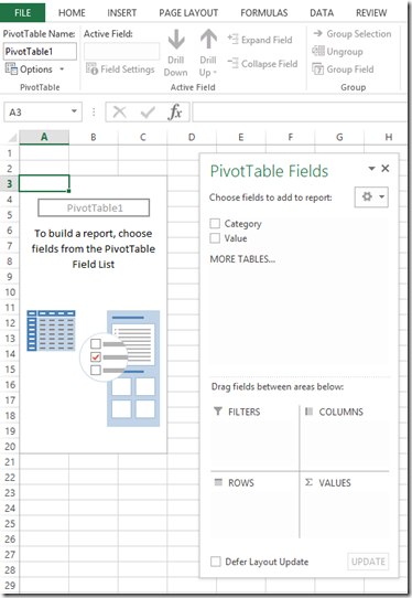 Tthen drag and drop your row categories to the rows section of the PivotTable Fields dialog box and also dragging your values to the values section:
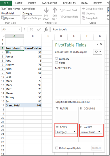 Your PivotTable will now have Values grouped in Rows.
2) Set Pivot Table Filter for Top or Bottom Values
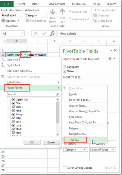
Now that we have data in our PivotTable, we can now set up our Value Filters to only show the Top 5 Values. To do this, select the Row Labels Drop Down Filter and then choose the “Value Filters” from the Drop Down List and then finally choose the “Top 10…” menu item.
Now this may seem strange since we only want the Top 5, but don’t worry, you get to change that next. After clicking on the Top 10… menu item, you can change the value from 10 to 5 and then press OK button.
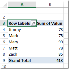
 Your PivotTable will now only display the top 5 results as you see here:
3) Create Pivot Chart
Now that we have our data set, you can create a Pivot Chart from the PivotTable and it will only display the filtered values.
You can do this by selecting any cell in the PivotTable and then Click on the Insert Ribbon and then choose the Pie Chart button from the Chart Group:
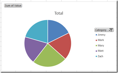
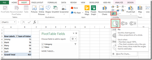 You will then see your Dynamic Pivot Chart created for the Top 5 values only.
 You are not limited to the Top X. You can also create another PivotTable and show the Bottom X as well back in step 2 and then change what you show in the Top 10 Filter:
4) Refresh Pivot Table Data
Now anytime you get a new data set or change the data set, to get an updated Pie Chart, all you have to do is Refresh your PivotTable and your chart will dynamically change.
You can refresh your PivotTable and Pivot Chart by selecting the Data Ribbon and then Choose Refresh All from the Connections Group.
Also, Excel will take care of any ties in the data, so if you have more than 5 in your top 5 due to ties, Excel will display the correct amount of items in your Pivot Table and Pivot Chart.
In this example, i have 6 values that are in the Top 5 due to ties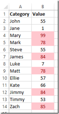
Rank 1=99
Rank 2=85
Rank 3=84,84
Rank 5=78,78
So when I refresh my data, I will get six Pie Slices instead of 5 as you see here: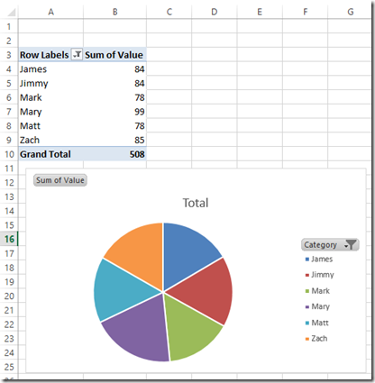
Hopefully that helped the person in need and you when you want to create a Top X or Bottom X chart. Simply put it into a Pivot Table and change the Value Filter.
Video Demonstration
Here is a quick video tutorial on the step-by-step process:
Free Sample Pie Chart Template Downloadable File
Here is a file that you can use to try it out for yourself. Simply open up the file and change some of the data points and then Refresh the PivotTable and see the results.
Dynamic Pivot Table Pie Chart Top X Values
Do you use the Top and Bottom Values filter in Excel Pivot Tables and Charts? Leave me your best use case in the comments below.
Steve=True

