When you build your Excel Dashboard, you will frequently want to use Conditional Formatting to create color callouts and other table based dashboard components. For instance, I used the conditional formatting in a Tiger Woods Graphic that I created to show his Wins, Top 10 Finishes vs Tournament Entries in Excel.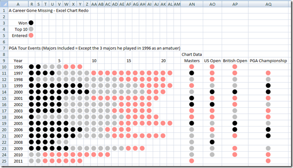 All of this was done using Excel Conditional Formatting.
When I started using these features in Excel, I was able to create basic conditional formatting that was already set up in Excel very quickly. However, I was very confused on how to create my own Conditional Format Formula Rules.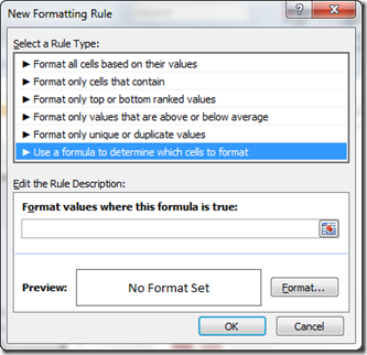
Then I found the trick and now I am going to share that tip with you.
The Problems:
1) How-to Write a Conditional Format Rule Formula – What does it need to return/do/equal?
2) How-to Write a Conditional Format Rule Formula that handles an entire range.
Have you had a similar problem/lack of Excel knowledge?
The Solution:
Then I finally figured it out.
1) The first TRICK to writing conditional format rules and formulas is to:
HIGHLIGHT YOUR RANGE AND THEN WRITE THE FORMULA IN TERMS OF THE TOP LEFT CELL IN THE RANGE.
That is it. Just write the Excel Custom Conditional Rule Formula in terms of one cell and then Excel applies that formula to every cell that you have added to the conditional format range. I don’t know if this caused you headaches and misunderstandings with Excel, but it did for me. If someone had just told me that, it would have saved me a lot of time and would have helped me immensely.
2) The second TIP is to write your conditional formatting rule so that it compares something and either returns a TRUE or FALSE.
Yep, that is right. We don’t need to return a value but instead we need to compare something and if it is
TRUE = the conditional formatting rule will apply and the formatting from this rule will be applied.
FALSE = the conditional formatting rule will not apply and no formatting from this rule will be applied.
The RULES of Creating Conditional Formatting Rules:
1) Write the formula as if the top left cell were the only cell being compared not the entire range.
2) Write the formula so that a TRUE or FALSE is returned
In Action:
Okay, at the bottom of this blog post is a FREE Excel Download File that contains all the Top 5 Baby Names both Female and Male from 1912-2011. That is like 100 Years! I found the data from the Social Security Administration: http://www.ssa.gov/oact/babynames/top5names.html
And things have changed over the years. However, when you look at all the 1000 names in the spreadsheet, your mind may start to spin. This would be a great way to create some conditional formatting to hide names that you don’t want to see.
As an example, the last 5 years of females names looks like this:
Now what if you wanted to only see all the names that begin with the Letter “E”?
That is a lot easier to see what names are popular based on what I care about. Turns out that my name “Steve” has never been in the Top 5 for the last 100 years ![]() . As a matter of fact, no Male name starting with “S” has made the Top 5 in the last 100 years. But plenty of Female “S” names have like Samantha,Sandra,Sarah,Shirley,Sophia andSusan.
. As a matter of fact, no Male name starting with “S” has made the Top 5 in the last 100 years. But plenty of Female “S” names have like Samantha,Sandra,Sarah,Shirley,Sophia andSusan.
I am not sure how you would do this with the standard Excel Conditional Formatting options. The available choices does not have an option for “Text that Starts with”.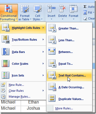
So looks like there are no rules and we need to create our own rule. Now time for the fun of it all.
Step-by-Step
1) Highlight the Range B6:K105
Highlight the range of cells that you want to apply this conditional formatting. You can always change this later if you would like. In this example, I will highlight the entire dataset of names that you see in the file download.
2) Create a New Conditional Formatting Rule
From the Home Ribbon, select the Conditional Formatting button from the Styles group and then choose “New Rule…” from the menu: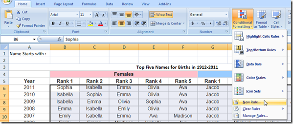
3) Select a Rule Type
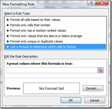
Click on the “Use a formula to determine which cells to format”
4) Write the Conditional Formatting Rule Formula
Remember, the rules of creating Conditional Formatting Rules:
1) Write the formula as if the top left cell were the only cell being compared not the entire range.
2) Write the formula so that a TRUE or FALSE is returned
What our formula needs to do:
a) Return True or False as the final answer
b) Compare the first letter of the cell to the value in Cell B1. We will use the LEFT function for this.
Now normally I would write an IF function, like this:
=If(left(b6,1)=$B$1,TRUE,FALSE) but this is overkill since Excel can always evaluate a formula comparison and return TRUE or FALSE. Therefore, we don’t need the IF statement. We can just use the “=” to compare the values.
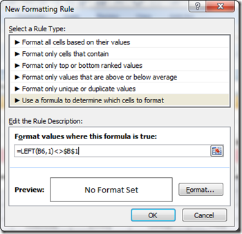
So, in the “Format values where this formula is true:” box, write the following formula:
This formula will return a TRUE or FALSE by looking at the first character in the text of cell B6 and if that character does not equal the value we put in b1. If it equals Cell B1’s value, then it is True, else it is False.
When it is FALSE, no Conditional Formatting will be applied to the cell.
When it is TRUE, the Conditional Formatting will be applied to the cell.
3) Set the Format for the True Condition
Okay, so now if the formula we just entered is true then we need to sent the format with the “Format…” button on the bottom right side of the “New Formatting Rule” dialog box.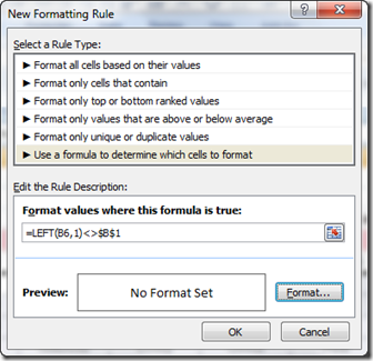
In our case when the formula is true that means that that it does not start with the letter we want. Therefore, we want to not show the value of that cell. Since we can’t remove the value, we can ‘fake’ hide the value of the cell. To do this, we need to set the format of the text in that cell to be the same as the cell color so that it looks like it has been removed.
So choose a Color of White from the Font Tab: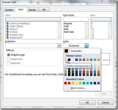
Your Conditional Formatting is now completed. You probably only see that all your values are probably gone/hidden. This is probably because you do not have any value in cell B1.
Once you put a letter in cell B1, you will then see some values appear and some are also hidden. For instance, if you put a “S” in cell B1, your spreadsheet will look like this: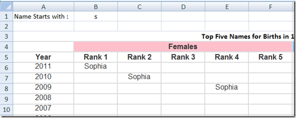
You can see that Sophia is now showing in the spreadsheet. If you investigate the other cells that appear blank by highlighting them in a range, you will see the values that are still there, but their format has been changed to a white font so they seem to disappear. See below if you squint very hard ![]() .
.
You may have to tilt your screen ![]()
So with this tip, you now know the tricks to writing a Conditional Formatting Rule. Hopefully that cleared up an confusion you may have had with righting these rules. Let me know in the comments all the interesting ways you have used conditional formatting in your Excel Dashboard Templates.
Video Tutorial
Free Sample Download Template File
Tips-and-Tricks-to-Writing-a-Conditional-Formatting-Rule-Formula.xlsx
Don’t forget to sign up for my RSS Feed so that you get the latest post and tutorial.
Steve=True

