Okay, for the last challenge, Peter went above and beyond and also submitted a VBA solution to this problem. Great job Peter!
Here is how it works:
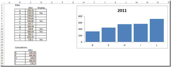
There is a data section, and a calculation section. The calculation section houses the rows that are hidden, and the chart is driven from this area. As soon as any changes are made to the data section, the calculation section (and chart) automatically update. Other than entering “yes”, there is no other operator action required. When a “Yes” is entered into column D, then rows are hidden in the calculation section, thus hiding the data section in the chart.
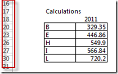
Notice that rows are hidden in the Calculations section by the VBA code:
Here is the VBA code:
Sub worksheet_calculate()
Dim MyRange As Range, C As Range
Application.EnableEvents = False
Set MyRange = Range(“Sheet1!c19:c30”) ‘Adjust range as needed.
For Each C In MyRange
C.EntireRow.Hidden = IsError(C)
Next C
Application.EnableEvents = True
End Sub
If you want to learn more about hidden cells in charts, check out these posts:
How-to Show Excel Chart Data and Keep Chart Size when Hiding Spreadsheet Columns and Rows
Video Demonstration:
Free Excel VBA Template File Download:
Friday-Challenge-on-Thursday-Only-Show-Selected-Data-points-in-an-Excel-Chart-VBA-Solution.xlsm
Also, come back tomorrow for another Dashboard challenge.
Steve=True


