In a previous Friday’s challenge, I presented the following user request.
Here was the question again and what you would have seen in the download file:
need help in getting a chart in an excel
Hi i have a problem, i want to get my report through getting how much total tally in each outlet, i want to get the AM for each outlet, PM total for each outlet and other all comparison of all total tally for all outlet, it can be charts or graphs or in pivot table. Thanks in advance. god bless.
Sample File: ballroom-occupancy_final.xls
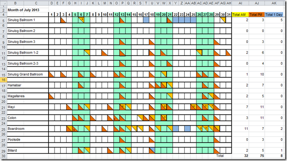
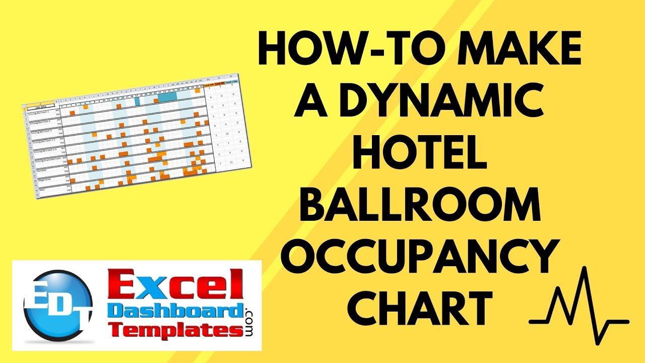
As you can see in the picture above, the Excel user is copying and pasting different colored triangles on each day so that they staff can quickly see when each ballroom is booked in their hotel. This can be very tedious for the user to copy and paste the upper right or lower left triangle to the right day and place. Also, because they are different colored shapes, the user has to manually count the hotel conference room usage. So how can we make all of this easier for the user? See below:
The Breakdown:
1) Setup the Data Layout
2) Create Dynamic Days of the Month
3) Create Conditional Formatting for Weekends and Hide Weekday Numbers
4) Create Conditional Formatting for Hotel Ballroom Usage
5) Create Hotel Room Count Formulas
Step-by-Step
1) Setup the Data Layout
Okay, this is one thing that I just wasn’t able to match exactly. You will notice that the user had one line per hotel ballroom. Since we can’t break up a cell into top right and bottom left, I had to expand each room into two rows (one for AM and one for PM). Along with that change, we needed to add an additional row for both the AM and the PM sections so that we can capture the extra information that the user wanted to see (Note the x that means that the booking is less than 4 hours and 2 means that the booking is consecutive over several days). Also, since each month may have up to 31 days, I had to expand the calendar to 31 days to accommodate that many days. Here is what your set up should look like for the daily data: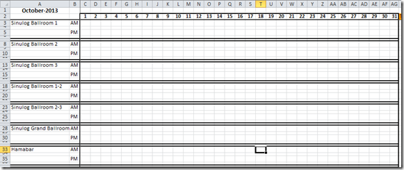
Now ewe are all set to create our new ballroom occupancy chart.
2) Create Dynamic Days of the Month
One of the manual tasks that the Excel user has to do on a monthly basis is figure out how many days are in the month for the chart they are building. Number of days can range between 28 and 31. Then there are leap year days. Since we are using Excel, lets see how we can make Excel do the heavy lifting for this operation.
a) Designate Cell A1 as the Date that Drives the Number of Days
We will enter in cell A1 a date so that Excel can calculate the number of days for each month. I have placed this custom number format in cell A1 so that the date entered only shows the Month and Year:
mmmm-yyyy
therefore, you will only see October-2013 when you enter an actual date of 10/1/2013 in cell A1.
b) In cell C1, you will need to enter this formula:
=IF(ISNUMBER(C2),WEEKDAY(DATE(YEAR($A$1),MONTH($A$1),C2),1),””)
Here is what this formula is calculating.
First, it checks to see if cell C2 is a number. =IF(ISNUMBER(C2),
If it is, then we will find the WEEKDAY
WEEKDAY(DATE(YEAR($A$1),MONTH($A$1),C2),1)
of the calculated Date from the Year of A1 and the Month of A1 and the value in C2. This will return a number between 1 and 7. The final number 1 at the end of the Weekday function tells Excel to calculate 1 as a Sunday and 7 as a Saturday.
Finally, if Cell C2 is NOT a number, then it will just display a blank in cell C1
,””).
We are using the cells in C1:AG31 to mark what the WEEKDAY is for this column. We will use this in a future calculation to display our Weekends for the current month.
Once you have entered your formula, you can then copy cell C1 all the way across to AG1.![]()
c) In cell C2, you will need to enter the following formula:
=IF(COUNT($B$2:B2)>0,IF(B2<28,B2+1,IF(LEN(B2)=0,””,IF(B2+1>DAY(DATE(YEAR($A$1),MONTH($A$1)+1,1)-1),””,B2+1))),1)
Lets look closer at this formula. First we are going to count the number of values starting in cell B2 and continuing on as we copy the formula right.
IF(COUNT($B$2:B2)>0,
So the next cell to the right will count cells B2:C2 and so on.
Now if the count in these cells are greater than zero, then we need to check the cell to the left and see if if is less than 28.
IF(B2<28,
If it is less than 28, then we are just going to add one to the value in the cell to the right as our final value in this cell.
IF(B2<28,B2+1
We can do this because all months in the calendar have 28 days or less. Next, if the value is greater or equal to 28, then we need to check the length of cell B2.
If it is equal to zero, then it means that we are in the first cell and we should just enter in a blank, but it also means we have an error and you will see that when no days show up.
IF(LEN(B2)=0,””,
If the length of the cell to the left does not equal zero, then we need to calculate the current day for this cell. To do this, we enter another IF statement
IF(B2+1>DAY(DATE(YEAR($A$1),MONTH($A$1)+1,1)-1),””,B2+1
and check to see if we add 1 to the cell to the left, will it be greater than the last day of the month for the month entered in cell A1. If it is greater than the last date of the month, then we want to just show a blank in the cell. If it is not greater than the last day of the month, then we just want to add 1 to the value in the left cell for this day. Once you have finished entering this formula in cell C2, you will need to copy it across to cell AG2:![]()
*****************************************************************
SIDE NOTE:
This is how you calculate how long any given month is: DAY(DATE(YEAR($A$1),MONTH($A$1)+1,1)-1)
This formula recalculates our date entered in cell A1 by adding one to the month assuming the date started at the 1st day of the month. Then subtracting one from that value and we find that day.
So if our date was entered as 10/1/2013, we add one month to this and get 11/1/2013, then we find the day of that value if we subtract 1 from 11/1/2013. If we subtract 1 from 11/1/2013, we get 10/31/2013 which is the end of the month for our value entered in cell A1. Then if we find the day of that date, we get 31 as our value.
*****************************************************************
So now we have created formulas where we can enter any date in cell A1 and our table/chart will fill in with the correct number of days for any month. Download the spreadsheet and try entering in this date in cell A1:
2/1/2016
You should see that this is a Leap Year and you will see 29 days in the month displayed with blanks after 29:![]()
3) Create Conditional Formatting for Weekends and Hide Weekday Numbers
Okay, now that you have calculated all the Weekdays for the current month in Cells C1:AG31, we can use this to calculate what day is part of a weekend. We are going to highlight all the days that are part of a weekend by using Conditional Formatting.
If you want to learn the trick to conditional formatting an Excel spreadsheet, check out this post and video:
The Tricks to Writing a Conditional Formatting Rule Formula
So to create highlight our weekends, first highlight the range of C2:AG66. Then click on the Conditional Formatting button in the Styles group on the Home Ribbon and choose the “NEW RULE…” menu choice: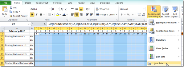
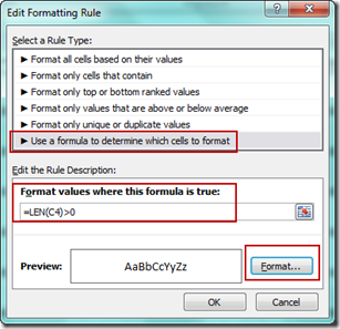
Then from the Edit Formatting Rule dialog box, choose the “Use a formula to determine which cells to format” in the “Select a Rule Type:” area.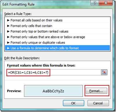
Then enter this formula
=OR(C$1=1,C$1=6,C$1=7)
(This formula is looking at cell C1 and if it equals a 1, 6 or 7, then it will consider this part of the weekend. I am matching the Excel user’s question to show Friday, Saturday and Sunday as part of the weekend. If your weekend is just on Saturday and Sunday only, then your formula would look like this:
=OR(C$1=1,C$1=7)
into the “Format values where this formula is true:” box and also change the cell fill color from the “Format” button to a light blue. Then press the Okay button and the Apply button on the next dialog box.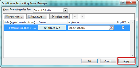
Your chart range should now have the weekends highlighted in a light blue fill color: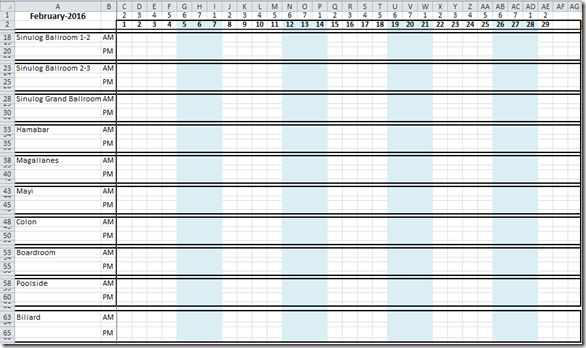
4) Create Conditional Formatting for Hotel Ballroom Usage
Now we need to give the user a visual cue when a hotel ballroom is booked either in the afternoon or the morning or for the whole day. We will also use Conditional Formatting for this visual display.
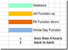
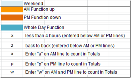
Now here is how we will highlight when a ballroom is booked in the hotel. Orange will represent a booking for the AM, Dark Brown will represent a PM function and Dark Blue will represent a Whole Day function. Users will do this by entering a “a” in the ballroom AM row, a “p” in the PM row and a “w” in the AM row to create the respective highlighting. Below the AM or PM rows, they can enter more details like the X or 2. Here is the legend/instructions on how to create the highlighting.
So to create highlight our booked dates, first highlight the range of C2:AG66. Then click on the Conditional Formatting button in the Styles group on the Home Ribbon and choose the “NEW RULE…” menu choice:
Repeat the step above for all the conditional formatting you see in this section.
a) AM Highlighting
From the Edit Formatting Rule dialog box, choose the “Use a formula to determine which cells to format” in the “Select a Rule Type:” area.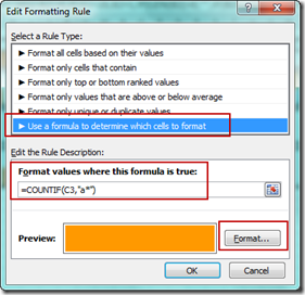
then enter this formula:
=COUNTIF(C3,”a*”)
And choose a color of yellow for the Fill color from the format button and a font color of yellow so that the “a” is hidden on the sheet.
b) PM Highlighting
From the Edit Formatting Rule dialog box, choose the “Use a formula to determine which cells to format” in the “Select a Rule Type:” area.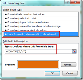
then enter this formula:
=COUNTIF(C3,”p*”)
And choose a color of brown for the Fill color from the format button and a font color of brown so that the “p” is hidden on the sheet.
c) PM Highlighting
From the Edit Formatting Rule dialog box, choose the “Use a formula to determine which cells to format” in the “Select a Rule Type:” area.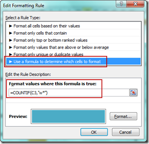
then enter this formula:
=COUNTIF(C3,”w*”)
And choose a color of medium blue for the Fill color from the format button and a font color of medium blue so that the “w” is hidden on the sheet.
d) Informational Text Color
The final conditional formatting needed is to highlight smaller informational rows (i.e. C4:AG4, C6:AG6, C9:AG9, etc). What we need to do is to show any text in these cells in a black format so that you can see them as our other conditional formatting will hide any text as we matched the font color to the cell fill color. You can do this for each row individually.
First, select the range of C4:AG4 and then click on the Conditional Formatting button. Then choose a new rule and put in this formula:
and choose a font color in the format button as a black font color.
After doing all of these steps, your Hotel Booking chart will look like this: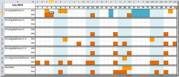
To fill in the colors for each day, the Excel user doesn’t need to copy and paste any shapes any more. They just have to go to the right day and time and enter either a “A” or “P” or “W” and Excel will do the rest using custom formatting. And now we can also use these values to count how much the Hotel Ballrooms are utilized with the CountIF function.
5) Create Hotel Room Count Formulas
In the cells to the right of each conference room, we just need to enter these formulas to count the usage that the user wanted
AH3 =COUNTIF(C3:AG3,”A*”)
AI3 =COUNTIF(C5:AG5,”p*”)
AJ3 =COUNTIF(C3:AG3,”w*”)
Copy these formulas down to each of the other conference rooms and you now have your final chart: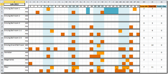
Video Tutorial:
Free Download Excel Template File:
Hotel-Ballroom-Schedule-Template1.xlsx
(Thanks to Pete for helping me pretty up my Excel Dashboard Template that you can download here)
Also, thanks to Don and Pete for sending in their solutions. They were quite similar to mine. Keep them coming! Please let me know in the comments on what you think about this template and if you can use any of it for your Excel charts.
Steve=True

