In my last post, Think-like-a-database-designer-before-creating-an-excel-dashboard-chart
we described the best way to configure your data to easily create your next dashboard.
In this post, we explore the use of Excel Slicers for your next dashboard project.
What is an Slicer?
Slicers scare some people, but they are simple and easy to use and oh so cool. Just think of them as a better filter.
Slicers are great because they filter data visually in your Excel workbook. Slicers will make it faster and easier for average users to filter Tables, PivotTables, PivotCharts, and cube functions.
Slicers were first introduced in Excel 2010. In that version of Excel, they could only be used with Pivot Tables.
In Excel 2013, they can also be used with Excel Tables.
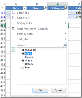
In a Nut Shell, Slicers move Everyday (hard to see) filters, into an easy to understand, see and use visual display for your Dynamic Dashboard Charts.
To This: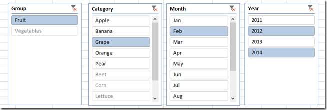 Now imagine your users using the very visual Excel Slicers to pick the data on their own to slice and dice your dashboard chart.
The Breakdown
1) Create a Pivot Table (2010 or greater) or Excel Table (2013 or greater)
2) Click in Table and Add Slicers
3) Select Slicer Filters
Step-by-Step
1) Create a Pivot Table (2010 or greater) or Excel Table (2013 or greater)
You can create an Excel Table in 2010 or 2013, however, only Excel 2013 will allow you to use slicers on the table. In any case, highlight the data table that you have created 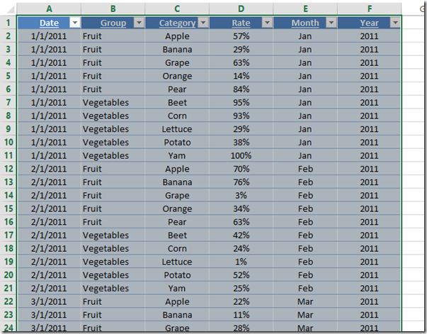
a) To Create an Excel Table
To create an Excel Table, then click on the Insert Ribbon and then choose Table from the Tables Group: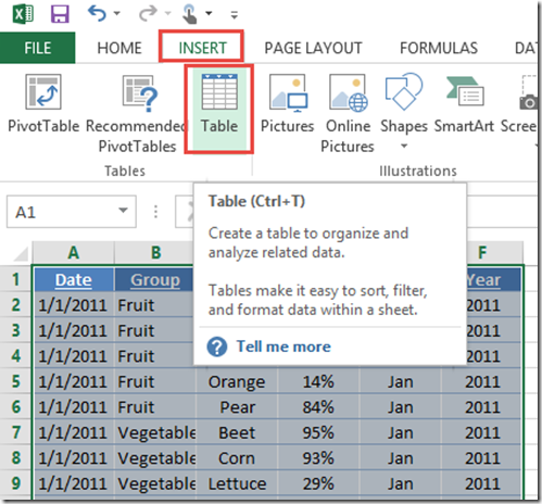
b) To Create an Excel Pivot Table
In both Excel 2010 and Excel 2013, you can add a Slicer to your Pivot Table. In order to do this, first, create your Pivot Table by selecting the Insert Ribbon and then Choosing Pivot Table from the Tables Group: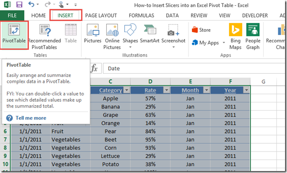
2) Click in Table and Add Slicer
Now we can add our slicers. You can do this in one of 3 ways:
a) Select the Excel Table or Excel Pivot Table and then select the Insert Ribbon. Then choose Slicer from the Filters Group:
b) For Excel Tables, select the Table and then then select the Tables Design Ribbon. Then choose Insert Slicer from the Tools Group: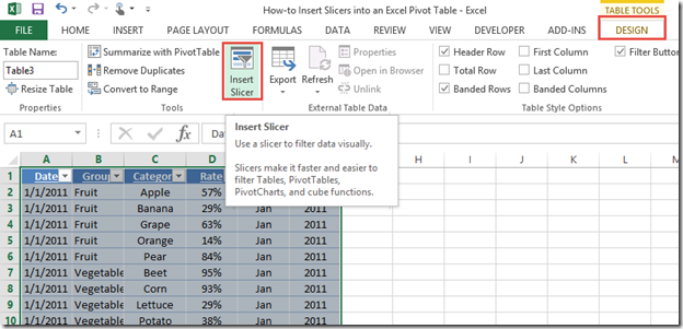
c) For Pivot Tables, select the Pivot Table, then Select the Analyze Ribbon, and then choose Insert Slicer button from the Filter Group: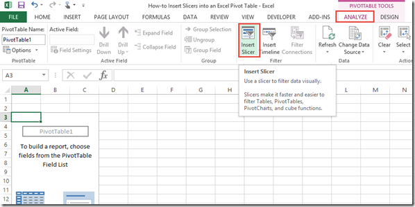
3) Select Slicer Filters
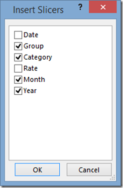
After completing the previous steps, you will then see the Insert Slicers pop-up menu where you can select the categories to filter. You probably only want to select the ones that are grouped categories instead of individual values.
Simply check the boxes of the filter categories you want to show and then press the Okay button.
Your Slicers will now appear in your spreadsheet as you see here: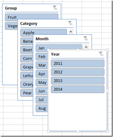 You can move and position the Excel Slicers as you see fit.
You may think that these are not better than Filters, but the real benefit of Slicers will appear when we create our final Excel Dashboard. They are so much easier to use for your dashboard viewers.
BONUS TIPS:
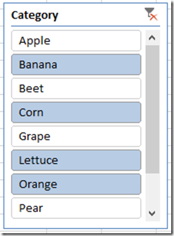
1) You can use your SHIFT KEY to select multiple contiguous values in your Slicer.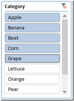 2) You can use your CRTL Key to select multiple non-contiguous values in your Slicer.
Video Tutorial
Check out a video demonstration on how-to add an Excel Slicer into your next Pivot Table or Excel Data Table here:
Sample File
Here is sample file download with a data set already created where you can create your own Excel Slicers:
How-to-Insert-Slicers-into-an-Excel-Pivot-Table.xlsx
Do you use Slicers on your Tables in your Excel 2013 Spreadsheets? Let me know in the comments below.
Steve=True

