In honor of Halloween I thought I would post something fun. For those that are not in the USA, Halloween is where children dress up in costumes and go door to door to beg for candy. ![]() Halloween always reminds me of spiders webs because people will decorate their property with spider webs. So I thought how can we create something that is Halloween-y in Excel.
Halloween always reminds me of spiders webs because people will decorate their property with spider webs. So I thought how can we create something that is Halloween-y in Excel.
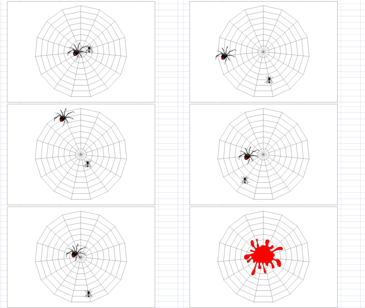
So I came up with this Radar Chart that changes as you press Recalculate in Excel. To Recalculate a spreadsheet quickly, you just have to press F9. As you can see by the animated GIF above, the spider and the fly move randomly around the Excel Radar Chart that I made to look like a spider web as I pressed F9.
The Breakdown:
So how did I do this? I used the following – Radar Charts, RandBetween Function, Custom Markers and NA() to create an Excel chart that changes when you hit recalculate.
You can see another example of Radar Charts on this Link:
How-to Highlight or Color Rings in an Excel Radar Chart
You can see another example of the Power of NA() in Excel Charts on this Link:
How-to Hide a Zero Pie Chart Slice or Stacked Column Chart Section
You can see another example of Creating Custom Chart Markers in Excel Charts on this Link:
How-to Make and Add Custom Markers in Excel Dashboard Charts
You can see another example of using RandBetween Function in Excel Charts to create data on this Link:
How-to Quickly Mock-up Data for a Dashboard Template
Step-by-Step:
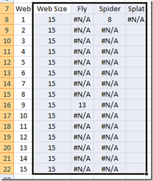
Step 1: Create your Data as follows (Note you can download the file at the end of the article):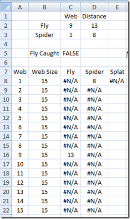
Cells C2:D3 contains this formula =RANDBETWEEN(1,15) These represent the location of the spider and the fly on the Radar Chart. Using the RandBetween Function will update their positions on the web (radar chart) when you press the Recalculate button in Excel which is F9.
Cell C5 contains the formula =AND(ABS(C2-C3)<2,ABS(D2-D3)<2) which I use to determine if the fly is caught and thus show the RED SPLAT instead of the spider or fly when it equals true. I just decided that if they were within 2 locations of each other, then show the splat since the 2 graphics will be really close.
Cells A8:A22 are just increasing numbers from 1 to 15. We will use these numbers to find the position of the spider or the fly.
Cells A8:A22 are just a fixed number of 15. We will use these numbers to create the web of the Radar Chart.
Cells C8:C22 contains the formula =IF(AND($C$2=A8,$C$5=FALSE),$D$2,NA()) Enter into C8 and then copied down to C22. This will set the position of the Fly in the Radar Chart.
Cells D8:D22 contains the formula =IF(AND($C$3=A8,$C$5=FALSE),$D$3,NA()) Enter into D8 and then copied down to D22. This will set the position of the Spider in the Radar Chart.
Cell E8 contains the formula =IF($C$5=TRUE,0,NA()) If the Fly is Caught = True then it will show the Splat graphic.
Step 2: Create the Web (Radar Chart)
Highlight Cell B7:E22
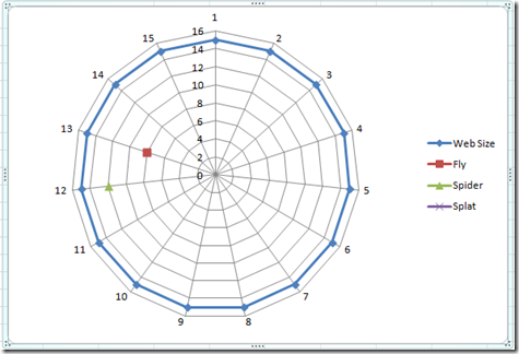
Select the Insert Ribbon and then choose the Other Charts from the Charts Group and then choose a Radar with Markers chart.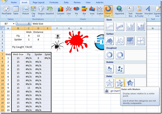
Your chart should look like this:
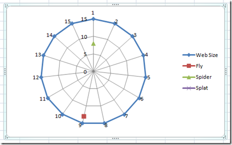
Step 3: Clean up the Excel Chart Junk and Change the Line, Remove the Numbers, Change Axis Labels to None and change the Websize series to No Line and Marker Options of None.
1) Click on the Legend and press delete
2) Right Click on the Websize line and select Format Data Series…
a) Change the Marker Options to None
b) Change the Line Color to No Line
3) Select the numbers on the outside of the last ring like number 6 and press the delete key.
4) Right click on the Axis labels (numbers that run up and down), and choose Format Axis. Then change the Axis Labels to None. NOTE: do not hit the delete key or the lines that run from the center out will disappear.
Your chart should now look something like this: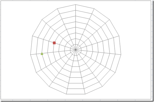
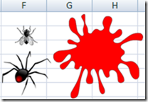
Step 4: Find some graphics of a spider, a fly and a red splat and insert those graphics into your spreadsheet. You can do this from the Insert Ribbon and then press Picture button in the Illustrations group.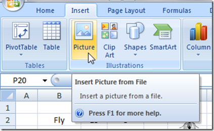
Here is what mine looks like:
Step 5: Change the markers in your radar chart to the markers you just inserted into the Excel Spreadsheet.
1) Select a graphic and copy it.
2) Select the Marker that it represents in the Radar Chart.
3) Press Control + V to paste it. (CTRL+V)
4) Repeat for each marker.
If you are having trouble finding the Splat series, either change the formula to a number so you can see it or check out this post.
How-to Select Data Series in an Excel Chart when they are Un-selectable?
Your chart should now look something like this: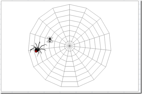
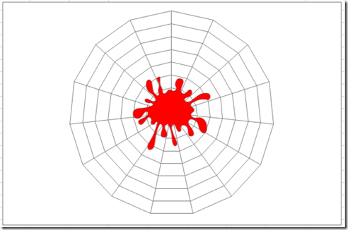
When the spider is close to the fly, your chart should look like this:
Video Tutorial:
Here is a FREE video tutorial demonstrating this technique:
SAMPLE EXCEL FIL
You can download a FREE sample file of Excel Chart to see how it works here:
Excel-Spider-and-Fly-Web-Worksheet.xlsx
I hope you and your family have a safe Halloween.
Steve=True

