I have been doing an excessive amount of data migration on my last assignment using Microsoft Excel. Typically I can do this so much faster in Excel than in most other programs including Microsoft Access databases. The new Excel can handle so much data that I can typically perform all the actions that I need as well as handle the calculation for most average data migrations.
In almost every data set I need to break up the text into many columns of data. For instance, some times an address is presented in the data within one cell but I need it to be in separate columns. This typically happens with names or addresses. In my example below, I will show you how to do this on an Address text string that is entered in one cell, but needs to be separated into multiple cells in Excel.
Now typically to break up an address from one cell to multiple cells, I almost invariably start by creating a formula.
For instance, for the picture above, if you data was this:
B2 = 1234 Main Street, Denver, CO 80202
(Note that there are 2 spaces after CO and before the postal code)
I would create the following formula to find the string of text that is for the street and place it in cell c3:
C3 =LEFT(B3,FIND(“,”,B3)-1)
I would use a nested Excel Formula of Left Function combined with Find Function. The Left function will get the text from the start of a string and also a specified number of characters. We specify how many text characters for Excel to get by finding the first comma using the the Find function and then subtracting one character from that function so that we do not include the comma.
In Cell F3, I would use a the Right Function in Excel. This is because in the United States the basic zip code is only 5 digits long. So a simple Right function is fine in this case.
F3 =RIGHT(B3,5)
Sometimes though, a zip code has 9 digits separated with five digits on the left of a dash like this: 80202-9988. If the data had both the 5 digits version and the 9 digit version, then we would have to use a nested If statement combined with both the Left and Right Excel Functions in the formula.
F3 =IF(LEFT(RIGHT(B3,5),1)=”-“,RIGHT(B3,10),RIGHT(B3,5))
Now here is where it gets real tricky. You have to use a more complex formula to get the City and State from B3 in order to separate the text from one cell to multiple columns. For the City text, we will use the MID function in Excel which will return text in the middle of another text string. So we are going to do the Mid of B3 with the starting from argument by finding the first comma in B3 plus 2 characters so that we do not return the comma and the following space. Next we will find the how many characters argument by finding the next comma after the first comma and then subtracting that number from the first comma position and also subtracting 2 to not show the comma and an extra space. Your formula to return the City from the Address would look like this:
D3 =MID(B3,FIND(“,”,B3)+2,FIND(“,”,B3,FIND(“,”,B3)+1)-FIND(“,”,B3)-2)
Wow, that was a tough one and took a few minutes to trouble shoot the formula.
Now for another tricky one of the State.
In this example, the state is only 2 characters, so I would use this formula to retrieve the state from the address cell. It is a nested IF Statement that checks to see if the US zip/postal code is 5 or 9 digits by looking for the dash as the fifth character from the right. If the formula finds a dash, then it will use the MID function in Excel to get the 2 state characters by finding the length of the text and subtracting 13 characters as the starting point. If it is only a 5 digit postal code, then it retrieves the 2 state characters by starting the MID function at the length of the text string minus 8 characters.
E3 =IF(LEFT(RIGHT(B3,5),1)=”-“,MID(B3,LEN(B3)-13,2),MID(B3,LEN(B3)-8,2))
Note, that my data has 2 spaces before the zip code and that this only works if there are 2 spaces before the zip code. What if there is only one space? Then your formula would have to be adjusted as follows to only go back 12 or 7 characters instead of 13 or 8:
E3 =IF(LEFT(RIGHT(B3,5),1)=”-“,MID(B3,LEN(B3)-12,2),MID(B3,LEN(B3)-7,2))
Now what if your states are not in the 2 character abbreviation format that most addresses use? What if your data has the entire state name? Well then we would have to make a more complicated formula much like we did with the City.
E3 =IF(LEFT(RIGHT(B3,5),1)=”-“,MID(B3,FIND(“,”,B3,FIND(“,”,B3)+1)+2,LEN(B3)-13-FIND(“,”,B3,FIND(“,”,B3)+1)),MID(B3,FIND(“,”,B3,FIND(“,”,B3)+1)+2,LEN(B3)-8-FIND(“,”,B3,FIND(“,”,B3)+1)))
Note, that my data has 2 spaces before the zip code and that this only works if there are 2 spaces before the zip code. What if there is only one space? Then your formula would have to be adjusted as follows to only go back 12 or 7 characters instead of 13 or 8:
E3 =IF(LEFT(RIGHT(B3,5),1)=”-“,MID(B3,FIND(“,”,B3,FIND(“,”,B3)+1)+2,LEN(B3)-12-FIND(“,”,B3,FIND(“,”,B3)+1)),MID(B3,FIND(“,”,B3,FIND(“,”,B3)+1)+2,LEN(B3)-7-FIND(“,”,B3,FIND(“,”,B3)+1)))
Copy the text example and formulas into a spreadsheet and give them a try. Make sure you put them in the same worksheet cells so that they will work without changing them.
AND NOW FOR SOMETHING COMPLETELY SIMPLER:
WOW, that seems real complicated. But don’t fear. You can either user the formulas I presented above or you can simply use the Text-To-Columns feature in Excel. I never knew about this feature for so long, and sometimes I forget to use it. This complex set of formulas can be easily accomplished in 3 easy steps. Here is how:
Copy your address text that you had in cell B3 and copy it to B8 so that you can then follow this example. Then Select Cell B8.
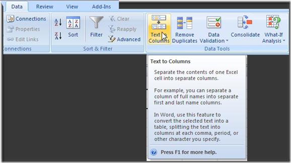
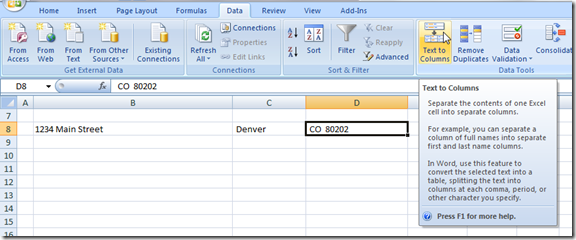
Step 1: Go to Data Ribbon and select the Text to Columns button does is that it separates the content in one Excel Cell into separate columns. The cool thing is that you set the way that it breaks up the data into those multiple columns.
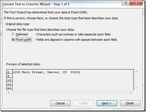
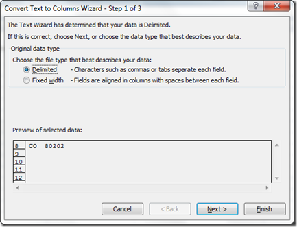
You can either choose a Fixed Width type from the Convert Text to Columns Wizard dialog box. This is best when you have a set number of characters from one of your data columns to the next. This was typical of older main frame data type. So for instance, if you may have 30 characters for the street and then the next 20 characters are the City and the next 2 are the state and the final 5 are the zip code. Then they would put in spaces for the streets and cities that didn’t fill up the character limits.
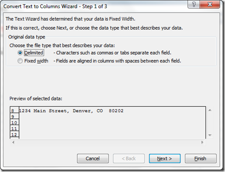
In our case, and in most cases today, you will see that the data is not a fixed width, but separated or “Delimited” by certain characters. So choose the Delimited radio button from the Convert Text to Columns Wizard dialog box and then hit the Next button.
Some separators are tabs or commas or semicolon or space. However, it is not always the case, so you can enter any character in the Other field.
Go ahead and select the Comma and in the Data Preview area of the Convert Text to Columns Wizard dialog box you will see this: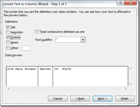
Now this doesn’t separate the Zip Code, but we will handle that in the final steps, so don’t worry.
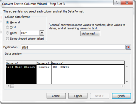
Go ahead now and press the Next button on the Convert Text to Columns Wizard and you will see the 3rd step that lets you set the Data Format for each column of data. You can now press Finish.
Your data will now look like this. It has been separated into columns from B8 to D8. But what can we do with the state and zip code? It is still in one column?
That is SO easy.
Step 2: Repeat the Text to Columns process by first selecting cell D8 and then go to your Data Ribbon and choose the Text to Columns button in the Data Tools group.
Then choose Delimited radio button from the Text to Columns dialog box and press Next button.
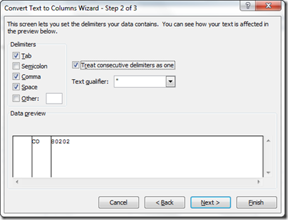
Now select the Space check box as a delimiter and also select the checkbox for the “Treat consecutive delimiters as one” so that you can take care of any double spaces that may proceed the zip code following the state.
Then press next and then the finish button and your data will now look like this:
Step 3: Now you may notice that we have one extra column, so the easiest step of the bunch would be to select column D and delete it. This is an extra column that was added when we chose the Space as a delimiter. No big deal.
Your final data will now look like this:
I suspect that it may take the average user 30 minutes to write the formulas but it takes less 30 seconds to use the Text to Columns features. So try and remember it and save yourself countless hours when working with your data.
VIDEO Tutorial:
Here is a video tutorial of using this technique on another set of data that needs to be split into 2 columns where the first column varies.
Please let me know if you have a more efficient way to break up an address from one cell in Excel to multiple cells in multiple columns by leaving a comment. Also, let me know what you thought about this post in the comments below. Finally, please let me know what types of content you would like to see on this blog in the comments. Thanks.
Steve=True


