In previous posts, I have espoused the virtues of the Pivot Tables in Excel and that you should always think in terms of a database programmer when you create your data layouts. If you missed those posts, you should check them out here:
Think Like a Database Designer Before Creating an Excel Dashboard Chart
How-to Insert Slicers into an Excel Pivot Table
How-to Create a Dynamic Excel Pivot Table Dashboard Chart
Class Exam Grade Excel Chart Using Slicers and a Pivot Table
But what if you have a large data set given to you and it is not in the proper format so you cannot easily create a Pivot Table from the data?
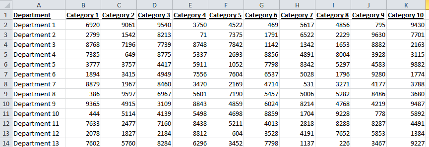
Your data layout was formatted this way:
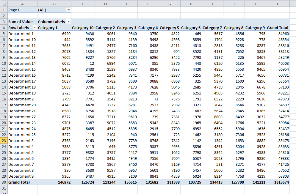
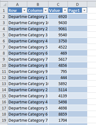
But you wanted the layout this way:
Well stress no longer, you can easily and quickly transform your Excel data into a Pivot Table friendly data set with this tip / trick.
The Breakdown
1) Launch the Classic Pivot Table Wizard
2) Complete Multiple-Consolidated Ranges Steps
3) Create Data Set from Drill Down
4) Rename Column Headers
Step-by-Step
1) Launch the Classic Pivot Table Wizard
To quickly transform your data, we need to use the “Multiple consolidation ranges” ability of the the classic “PivotTable and PivotChart Wizard”. If you are newer to Excel, you may never have known that this exists. I used it so much, I have memorized the keystrokes and that is what I use to create a Pivot Table on a daily basis.
To launch the Pivot Table Wizard, you will first need to press ALT+d and then let those keys go and press the “p” button on your keyboard. The PivotTable Wizard Dialog Box will then launch as you see here.
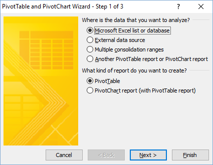
So remember, press the ALT and “d” keys together and then let go and press the “p” button.
2) Complete Multiple-Consolidated Ranges Steps
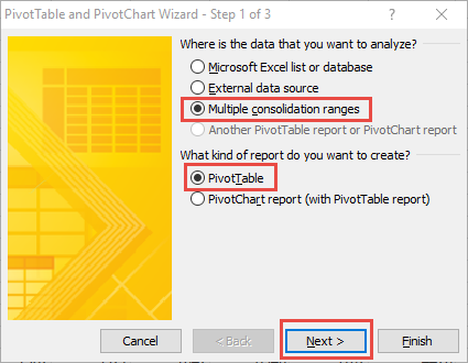
Now that we have the classic wizard open, you will want to make the following selections
a) Multiple consolidation ranges
b) PivotTable
and then press the Next button:
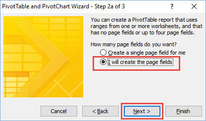
You will then see this dialog box for step 2a. Here you want to choose “I will create the page fields” and then press the Next button.
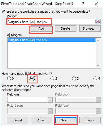
Step 2b will take a little more work. First, click in the Range field, then select your range on the spreadsheet. Once you have your data range selected, press the Add button. Your range will then be set in the All Ranges section. After you complete the range, you will then want to select the “1” radio button in the section “How many page fields do you want?” and then press the Next button.
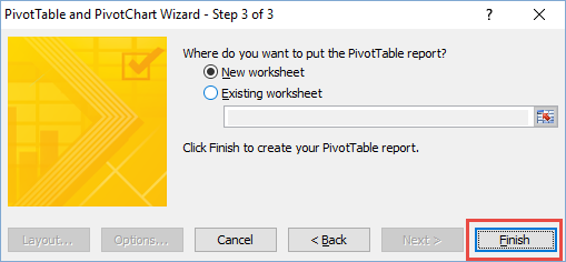
The final step is to choose where you want the final PivotTable to be created. You get to choose. Typically, I will just have it created on a new worksheet and then press the Finish button.
Your data will then be transformed into a PivotTable as you see in the next step.
3) Create Data Set from Drill Down
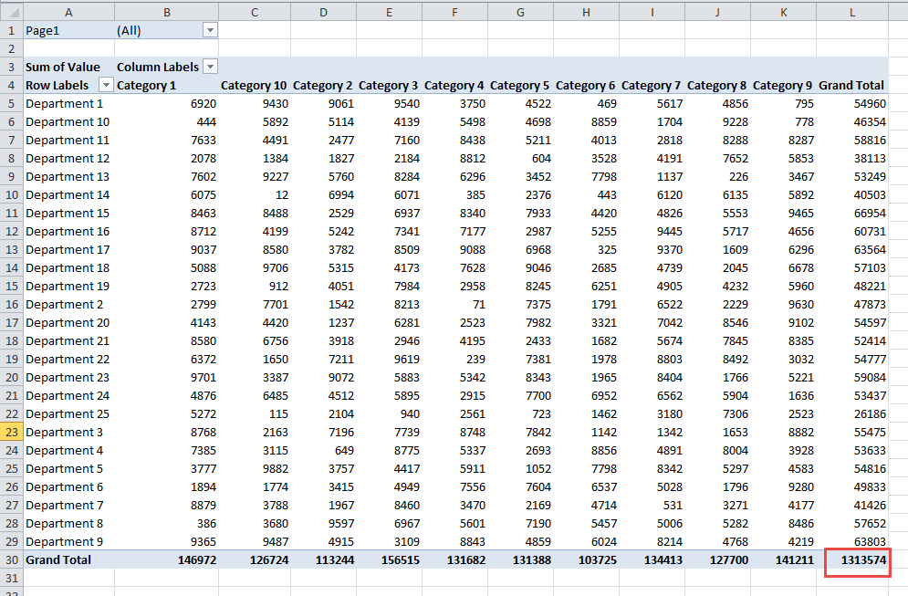
Even though the original data now looks like a Pivot Table, we don’t yet have our data in a Pivot Table format for adding and editing. In order to create the data like you would imagine generated this Pivot Table, we have one final step. You can drill down into any PivotTable and see the base data when you double click on any number in the table. So to get all of our data we want to Drill Down on the Grand Total for the entire Pivot Table in the bottom right corner.
4) Rename Column Headers
Once you have drilled down into the Pivot Table, your data will explode into a transformed data set as you see below. As the Pivot Table doesn’t really know the column headers that you started with, you will want to update cells in the first row to Department and Category
As you can see, it can take just a few minutes to transform your data when it would take you a long time to do it by hand.
Video Demonstration
File Download
Try it yourself with this sample Excel file:
How-to-Explode-a-Pivot-Chart-from-an-Existing-Data-Set.xlsx
Do you use the Insert Ribbon > Pivot Table or the Classic Pivot Table Wizard with Alt+d – p? Let me know in the comments below.
Steve=True


