Here is a quick demonstration on the technique that Peter used for his Step Charts:
Learn More about the Challenge HERE
To try it yourself as you watch the video, download this file and copy the formulas below:
Video Demonstration for this technique:
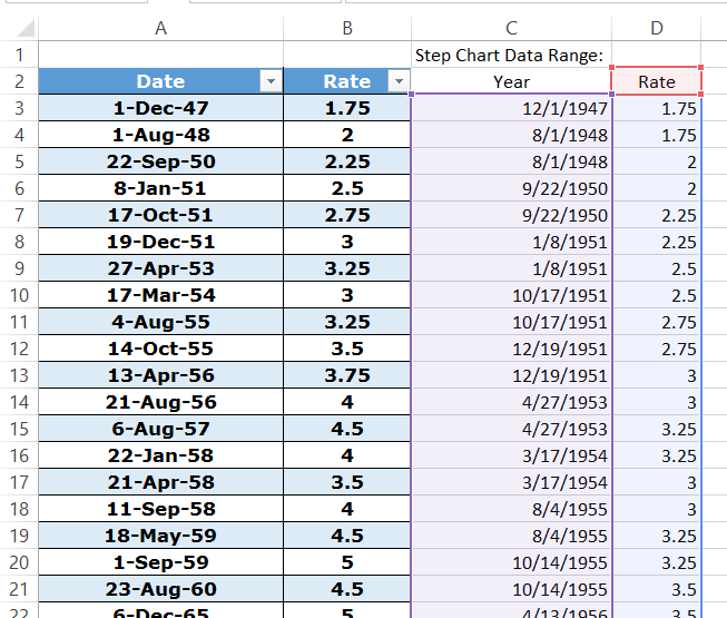
In Cell C3, Peter used an Array formula to create his step chart date data
=INDEX(Table13[Date],MATCH(INT(ROW(1:1)/2)+1,ROW(Table13[Date])-ROW($A$3)+1,0))
Enter this formula in cell C3 and then press CTRL+SHIFT+ENTER instead of just enter. It will then look like this in the formula bar:
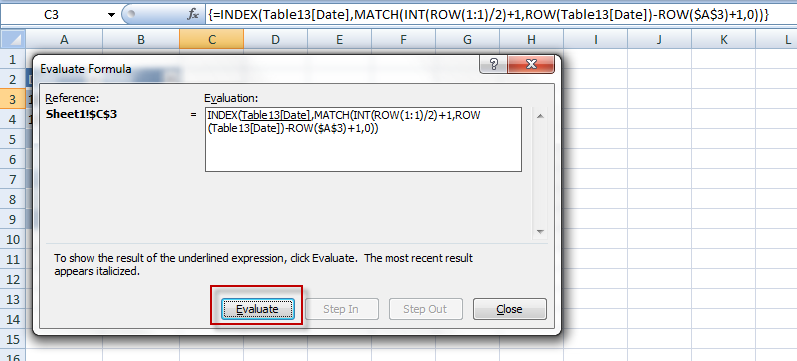
{=INDEX(Table13[Date],MATCH(INT(ROW(1:1)/2)+1,ROW(Table13[Date])-ROW($A$3)+1,0))}
If you want to see how this formula is working, go to your Formula Ribbon and press the Evaluate Formula button:
And jump thru the formula by pressing the Evaluate button and see that it is doing. You will learn a ton!
In Cell D3, for the rate data, Peter used a combination of index and match and the INT function to act as a counter that steps twice (i.e. 1,2,2,3,3,4,4,5,5,6,6,etc)
Enter this formula in cell D3, but no need to press CTRL+SHIFT+ENTER, just hit enter:
=IF(INT(ROW(1:1)/2)+1<>INT(ROW(2:2)/2)+1,INDEX(Table13[Rate],MATCH(C3,Table13[Date],0)),D2)
Then copy down the data to about row 700 where you will see #NA in several rows. Delete those rows.
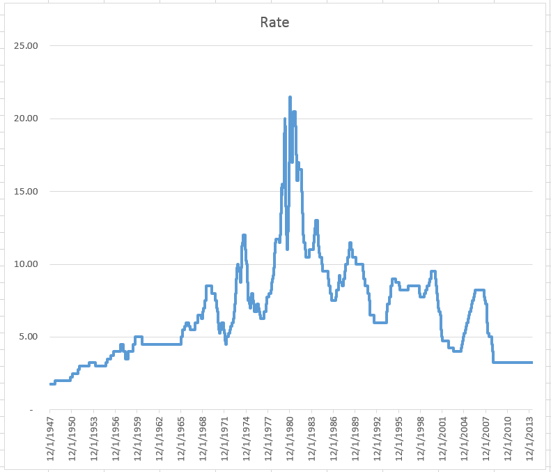
Then Highlight cells C2:D683 and Insert a line chart.
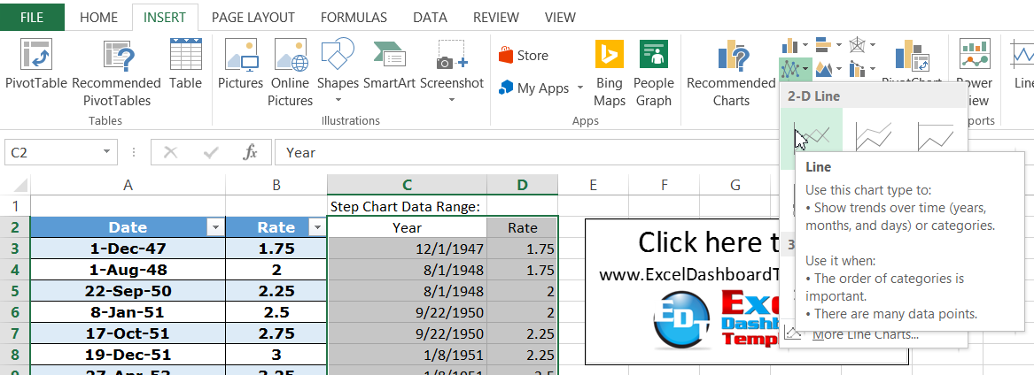
You will now have your fancy step chart all done for you.
Just remember, there is never one right way in Excel. Thanks Pete for showing us another way.
Steve=True


