In our last Friday Challenge, we were investigating Step Charts. In case you missed it, you can check it out and download the sample data file here:
Also, you should check out the quickest manual way to create a step chart here:
How-to Create a Step Chart in Excel with 3 Quick Steps
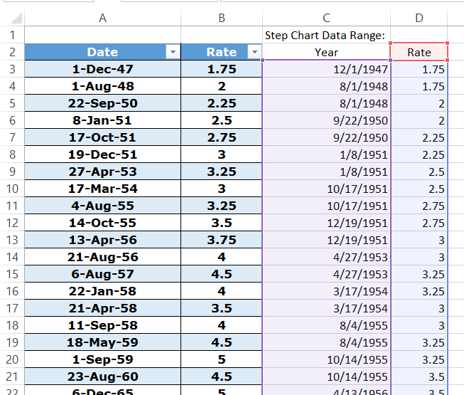
So in this post, we investigate a way to create your chart data with a formula. My functions of choice are SMALL and VLOOKUP. Check it out in the Step-by-Step, Video Tutorial and Free Sample File Below.
The Breakdown
1) Insert Formulas
2) Copy Down Until you see a #Num Error
3) Create Chart
Step-by-Step
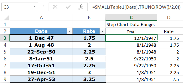
1) Insert Formulas
Note, this formula was written when your data starts when Date is in cell A3 / Year is in Cell B3. If your data is in a different cell, first copy these formulas to the cells described below, then copy and paste them to the final destination that you desire.
Copy formulas as shown below:
C3: =SMALL(Table1[Date],TRUNC(ROW()/2,0))
This returns the smallest value as designated by the Trunc(Row()/2) function of your data range. Trunc’ing the formula in Excel and then dividing by 2 will help you to repeat the same value in two consecutive rows. Check out the video below to see what I mean.
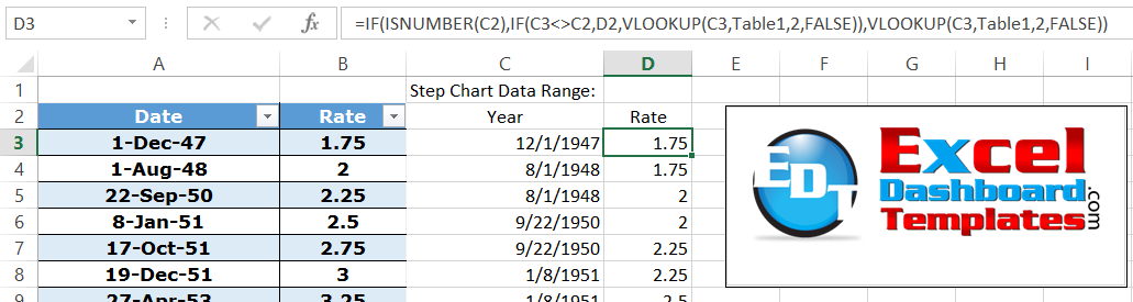
D3: =IF(ISNUMBER(C2),IF(C3<>C2,D2,VLOOKUP(C3,Table1,2,FALSE)),VLOOKUP(C3,Table1,2,FALSE))
This formula first looks to see if you are at the beginning of the data set. If the value in C2 is a number, then we are in the middle or end of the data set and you are then pushed into the second if statement. The second if statement looks to see if you are in the first or second repeating value that we need for the step chart. If C3<>C2, then we are in the second repeating value and we just need to return (repeat) the value of cell D2. If C3=C2, we are in the first of the 2 repeating values, then we need to look up the value of the date in column C. The final Vlookup looks at the first if statement and if it is not a number, then we need to look up the value in Column C.
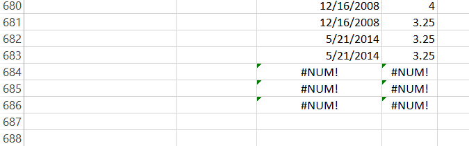
2) Copy Down Until you see a #Num Error
Since we need one chart data point for the first and last points and then we need two chart data points for each of the other ones.
For instance, in the Prime Rate charting challenge, we had 341 data points total. We therefore would need to copy the formula down past the original data for a total of 680 rows [ =(341-2)*2+2 ]. If you copy it down farther then that, you will start to see a value of #NUM in the cells as it has gone beyond the actual data.
3) Create Chart
Now you have your step chart data. You just need to highlight cells C2:D683 and then create a line chart from your insert menu.
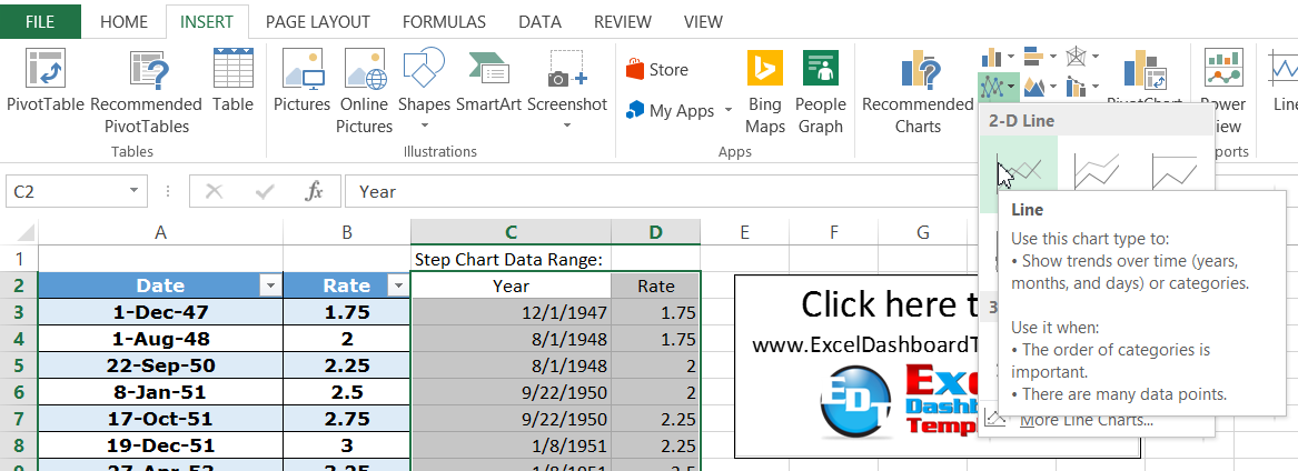
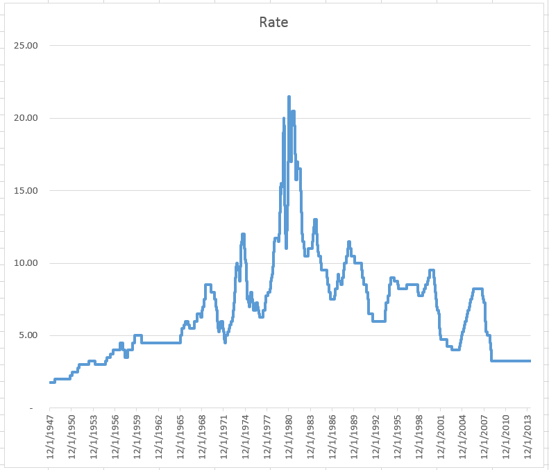
You will then have a perfect step chart made from VLookUp and Small Functions.
Sample File
You can see these formulas in action here:
Step-Chart-Friday-Challenge-Using-Small-Function.xlsx
Video Demonstration
Check out building these Step Chart formulas in Excel here:

If you have better formulas to create a step chart then please paste them in the comments section below.
Steve=True


