Yesterday, I posted the a demonstration on how to make a Step Chart in Excel.
You can check out that post here:
How-to Easily Create a Step Chart in Excel
However, the process of setting up the data was a manual process.
So I thought that we should post a Friday Excel Challenge to see how we can automate creating the chart data range.
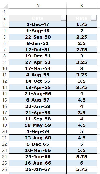
For this challenge, we will be using the history of the United States Federal Funds Rate (which is used in calculating the US Prime Rate). This data set has 341 data points, which would be very arduous to try and create the Step Chart data range manually.
The Challenge:
1) Download the US Prime Rate (Based on the Federal Funds Rate) data file.
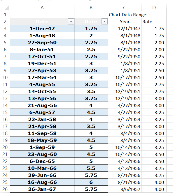
2) Write a formula for cell C3 that can be copied down to make the Step Chart date range that will be used for the horizontal axis.
3) Write a formula for cell D3 that can be copied down to create the Step Chart rate series.
4) Copy the formulas down columns C and D to make your chart data range.
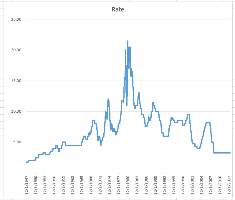
5) Create the Excel Step Chart
Here is a sample of what the original data series looks like:
Here is what your Excel chart data range will look like:
Here is a what your final Step Chart in Excel will look like:
Here is the Excel Spreadsheet with the Rate Data:
Step-Chart-Friday-Challenge-Data.xlsx
Submit your formulas in the comments section below (note that there is a delay of when you submit the comment and when you will see it on the website because I approve the comments to keep out spam bots).
It took me a few tries to make a really efficient formula. Good luck and come back next week to see the entries and also my demonstration on my technique. You can also download the final Excel file next week.
Thanks for your contributions in advance.
Steve=True


