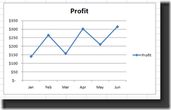
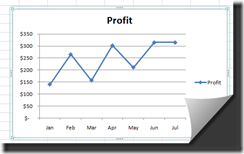
Wouldn’t that be awesome if Excel can just change my chart every month or week when I add more data? This can happen for you if you come to love the Offset function in Excel too.
So we have learned one way to make a dynamic chart in Excel for our Company Dashboard, but sometimes setting up your data table isn’t the right solution. So how else can we make a chart dynamic?
We can use the Offset function that Excel already provides for us. This is an incredible function and is perfect for Dashboard charts and graphs.
What is the Offset Function?
Here is what Microsoft Excel states for the Offset Function: “Returns a reference to a range that is a specified number of rows and columns from a cell or range of cells. The reference that is returned can be a single cell or a range of cells. You can specify the number of rows and the number of columns to be returned. OFFSET doesn’t actually move any cells or change the selection; it just returns a reference”
In short what does that mean for my dashboard? It means that you can let users define the data range that they want to see in a chart and you don’t have to modify the chart for the new data range. So if your users only want to see the last quarter of Sales for a chart or want to see the last year, they can pick the range they want to see and the Excel offset function will fetch and send the updated data range to your Dashboard Chart.
It also means that we can make formulas that automatically changes a chart when new data is added to a column or row of data. Therefore, you never have to modify your chart data series when you add more data. For instance, we just got new sales figures and would like to add the data to the spreadsheet and have the chart update itself to now include the new data point.
Syntax for the Excel Offset Function
=OFFSET(reference,rows,cols,height,width)
This is kind of like drawing a map for excel to fetch data.
The breakdown
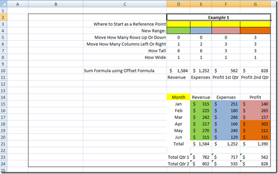
=offset( start where? , move up/down , move left/right , size down , size right )
Reference = Tell Excel where to start. This can be one cell or a range of cells.
Rows = Tell Excel how many rows to move the cell or range reference up or down. Positive numbers will shift the cell/range reference down and negative numbers will shift the cell/range reference up. If you don’t want to shift the range up or down, just leave this blank.
Columns = Tell Excel how many columns to move the cell or range reference left or right. Unlike VLookup, this can go left or right. Positive numbers will shift the cell/range reference right and negative numbers will shift the cell/range reference left If you don’t want to shift the range up or down, just leave this blank.
Height = Tell Excel how tall (in terms of rows) to make the cell or range reference. Positive numbers only. If you don’t want to change the size of the original Reference, just leave this blank.
Width = Tell Excel how wide (in terms of columns) to make the cell or range reference. Positive numbers only. If you don’t want to change the size of the original Reference, just leave this blank.
Examples:
Single Cell Reference starting point D9
Move down one cell: =offset(d9,1,,,) > (start at d9 result = d10)
Move up one cell: =offset(d9,-1,,,) > (start at d9 result = d8)
Move right one cell: =offset(d9,,1,,) > (start at d9 result = e9)
Move left one cell: =offset(d9,,-1,,) > (start at d9 result = c9)
Move down one cell and right one cell: =offset(d9,1,1,,) > (start at d9 result = e10)
Move down one cell and left one cell: =offset(d9,1,-1,,) > (start at d9 result = c10)
Move up one cell and left one cell: =offset(d9,1,-1,,) > (start at d9 result = c8)
Move up one cell and right one cell: =offset(d9,1,1,,) > (start at d9 result = e8)
Don’t Move but increase the range to 2 rows down plus the original cell =offset(d9,,,3,) > (start at d9 result = d9:d11)
Don’t Move but increase the range by 2 columns right plus original cell =offset(d9,,,,3) > (start at d9 result = d9:f9)
Don’t Move but increase the range by 2 columns right plus original cell and increase the range to 2 rows down plus the original cell =offset(d9,,,3,3) > (start at d9 result = d9:f11)
Move left 2 columns and up 2 rows and also increase the range by 2 columns right plus new starting cell and increase the range to 2 rows down plus the starting cell
=offset(d9,-2,-2,3,3) > (start at d9 result = b7:d9)
I HAVE THE POWER!!
That was fun, but how is this useful you might ask? Seems to take longer than just picking a new range.
The true power comes into play when you replace the numbers or the starting reference with formulas!
For instance, in a simple SUM formula, what if you use OFFSET to change the SUM range to add new values to the sum when they are added to a column?
Lets see how that works:
If I create a SUM formula using OFFSET, where I am counting the rows in a particular column, I can feed that count into the OFFSET Formula to return a range for the SUM function to add.
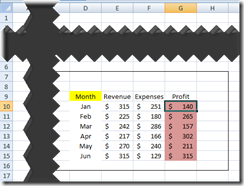
=SUM(OFFSET(G10,,,COUNT(G:G),))
The Breakdown:
= SUM ( this range { OFFSET = start at G10,
don’t move up or down, don’t move left or right,
increase the range down by the number of entries in Column G,
don’t increase the range by any columns wide } )
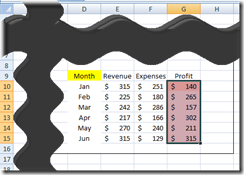
Since there are 6 entries in column G for this example: = SUM (G10:G15)
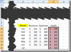
When we add one more entry to column G the SUM formula changes to =SUM(G10:16)
That is pretty cool. So now you know how to have Microsoft Excel return a Dynamic Cell Reference or Range of Cells that can be used in other formulas.
Now in the next post we will use the OFFSET Function to return a reference to a range of cells for our Excel Dashboard Chart in order to make it Dynamic.
Here is a Free Sample Excel Template using Offset Formulas:
Excel-Offset-Tutorial-Download.xlsx
Don’t forget to Sign up for my RSS or Email distribution for the next posting. Also, please leave me a comment on this posting or a posting you would like to see.
Steve=True


