So all the US news agencies keep talking about the Fiscal Cliff. This reminded me of a problem that many people have when making an Area Chart. Given this data: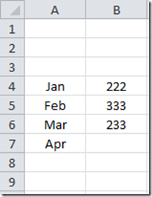
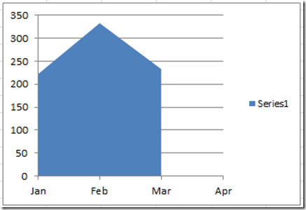
I have seen several posts where people want to make their area chart stop and show a cliff when there is a blank category value (notice that there is a blank in cell B7 that is part of the chart range). Much like this:
However, when they highlight the data range (Cells A4:B7) and create an Excel Area Chart they get this: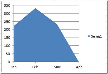
NOT what they wanted ![]() . It appears that Excel treats any Blank data point in an Area Chart as though it were a zero.
. It appears that Excel treats any Blank data point in an Area Chart as though it were a zero.
For Excel 2007 there is also a very fun Excel feature (maybe bug is the better term) in that when you create the area chart it shows a cliff, but when you save and open the file your cliff has fallen and it can’t get up.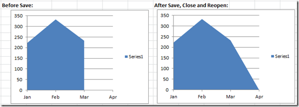
Well here is how to create your Area Cliff Chart in a step-by-step fashion and there is also a Video Tutorial link at the bottom of the page.
Step-by-Step
1) Create your Data Set for the Excel Area Chart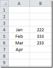
2) Create Area Chart
Highlight data range from A4:B7, then from the Insert Ribbon, press the Area button in the Charts group and then select the 2-D Area Chart: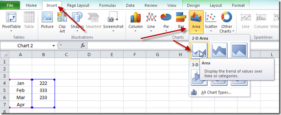
Your chart will now look like this (in Excel 2010):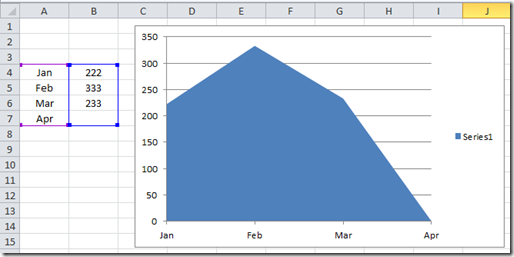
As you can see the Excel default is to treat Blanks in an Area Chart as a zero and draws the area from the previous category to the horizontal axis.
However, in Excel 2007, your graph will look like this, but don’t be fooled, if you save the file, close the file and reopen, your chart will look like the Excel 2010 version. You still need to follow the next steps.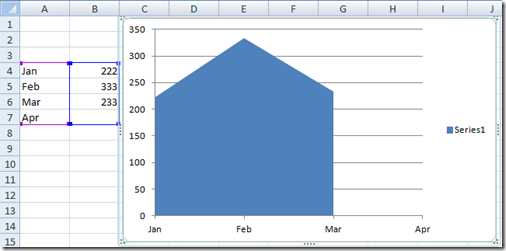
3) Change Select Data Option
Select the chart and from the Design Ribbon, choose the Select Data button from the Data group: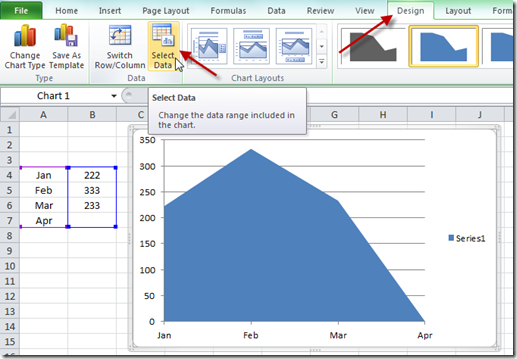
You will then see this Excel Dialog Box and you want to select the Hidden and Empty Cells button: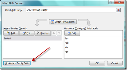
You will then see this Excel Chart Dialog Box: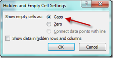
Excel 2010: You will want to select GAPS for the “Show empty cells as” radio button.
Excel 2007: You will want to select ZERO and then choose the GAPS for the “Show empty cells as” radio button again. I think that the Gaps selection you see is a bug and it is really has Zero chosen for you. If you do not do this, then your chart will default back to Zero when you reopen the file. IMPORTANT: So to reiterate this: When you create an Area chart in Excel 2007, even though the newly created chart shows a cliff and when you open the Hidden and Empty Cell Settings dialog box you see that Gaps are chosen. This will change when you save the file, close and reopen the file. To prevent this, open up the Hidden and Empty Cell Settings dialog box and then choose Zero and then Gaps for the “Show empty cells as”:” radio button. This will fix the issue.
And then your final chart will look like this for both Excel 2010 and Excel 2007: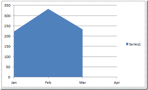
Look at that, we saved the U.S. from the Fiscal Cliff using Excel Charts and Graphs ![]() Make sure you sign up for the blog so that you are sure to get the latest posting.
Make sure you sign up for the blog so that you are sure to get the latest posting.
Video Tutorial
Here is the video tutorial demonstrating exactly how to create an Area Chart Cliff in Excel 2007 and Excel 2010:
Please make sure and sign up for my blog so you get the latest Excel Tip and Trick.
Steve=True

