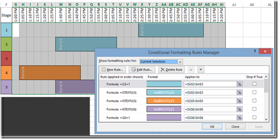
Recently, I saw an Excel User posting a question about how to make this Music Festival Schedule using Excel Charts.
However, he originally created the schedule in the worksheet area using cell fill colors and merge and center. But this can be a lot of work to adjust the schedule by moving and reformatting the worksheet cells.
.
In the next post, I will show you how to create this schedule using Excel Charts and Graphs (as per the users request), but for now, lets see how we can automate the schedule by using formulas and conditional formatting.
The Breakdown
1) Create Data and Conditional Chart Range
2) Create Array Formula
3) Copy Array Formula across the Conditional Chart Range
4) Create Conditional Formatting for Blank Cells
5) Create Conditional Formatting for Right End of the Bar
6) Create Conditional Formatting for Middle Bar Area
7) Create Conditional Formatting for Left End of the Bar
8) Adjust the Text Alignment to Vertical
Step-By-Step
1) Create Data and Conditional Chart Range
First we need to set up our Schedule Data and a range for the Conditional Formatting Bar Chart
I just placed my Conditional Formatting Bar Chart Area to the right of my Musical Schedule Data of what band is on what stage and the start and end times.
2) Create Array Formula
In Cell G2, we need to create this array formula
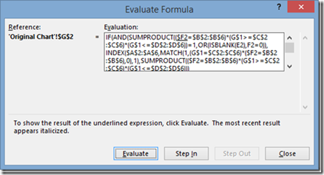
{=IF(AND(SUMPRODUCT(($F2=$B$2:$B$6)*(G$1>=$C$2:$C$6)*(G$1<=$D$2:$D$6))=1,OR(ISBLANK(E2),F2=0)),INDEX($A$2:$A$6,MATCH(1,(G$1=$C$2:$C$6)*($F2=$B$2:$B$6),0),1),SUMPRODUCT(($F2=$B$2:$B$6)*(G$1>=$C$2:$C$6)*(G$1<=$D$2:$D$6)))}
Now this is a normal formula that becomes an array formula by pressing CTRL+Shift+Enter when we are done creating it.
In layman’s terms, the formula is checking to see if a Band will Start playing at this Time on this Stage
….If yes, then find and insert the Band Name
….If No, then see if a Band is still playing on the stage at this time
……….If Yes, then insert a 1 for True or a 0 if False
Now lets break the formula down into its parts:
=IF(
AND(SUMPRODUCT(($F2=$B$2:$B$6)*(G$1>=$C$2:$C$6)*(G$1<=$D$2:$D$6))=1,OR(ISBLANK(E2),F2=0)),
in layman’s terms – See if a band will start playing at this time on this stage
IF 1) SumProduct = True (or 1) by checking if there is a band playing at the combination of the Stage F2 combined with the Time G1 equals a combination of the Stages and Times in Columns B and C
AND 2) Check and See if we are the right most cell of the formula range by checking to see if E2 is Blank OR Is the cell to the left of the current Cell=0 so that we will know if this is the Start of a Band’s playing time
If Yes, Then
INDEX($A$2:$A$6,MATCH(1,(G$1=$C$2:$C$6)*($F2=$B$2:$B$6),0),1),
in layman’s terms – Since this is the start of a bands playing time on this stage, find (Match) and return the bands name (Index) that will start playing on this stage at this time.
The complicated match formula is why we need to make this an Array Formula since we need to check 2 different criteria to return the right row for the band that is playing on this stage at this time. We need to check the Start time in C2:C6 and compare it to G1 and also check the Stage in Cell B2:B6 and compare it to F2. If all this matches, the Match formula will return the Row of the band name that starts playing at this time.
Else
SUMPRODUCT(($F2=$B$2:$B$6)*(G$1>=$C$2:$C$6)*(G$1<=$D$2:$D$6)))
in layman’s terms – This formula returns a True (1) or a False (0) value after checking to see if a Band is Playing on this Stage at this Time.
To create an array formula you need to press CTRL+Shift+Enter when we are done editing it.
To see how this formula works, download a copy of the spreadsheet and go to any cell in the Conditional Bar Chart area and then under the Formulas Ribbon, press the Evaluate Formula button and then Press the Evaluate Button to see how it works at each part of the formula.
Here are some more Tips about Array Formulas in Excel:
Removing Array Formulas Around Your Excel Charts and Dashboards
Protecting Your Excel Charts and Dashboards with Array Formulas
3) Copy Array Formula across the Conditional Chart Range
Now that we have the Array formula in cell G2, we need to copy and paste it to the rest of the Conditional Bar Chart area. NOTE: You cannot include the original cell that you created in the Array formula as it will show you an error that you can’t update an Array formula. So don’t include it in your paste area. You may need to copy and paste the Array formula across the row first. 
 And then copy and paste the Array row down to the other rows.
 You can now see that on Stage 1, Band D starts on 2:25PM and goes until 3:50PM. Also, no other bands are playing as there are all Zeros from the resulting If statement.
4) Create Conditional Formatting for Blank Cells
Now that we have our data laid out the way we need for our conditional formatting gantt chart, we can add the conditional formatting and the chart will come alive.
We need to do it in 4 parts.
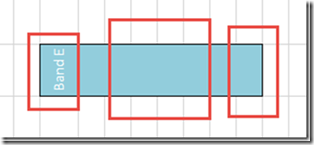
If look at the elements of the bar, you will notice that there are 3 parts to it and we will want to create a separate Conditional Formatting for each one of those parts
a) Left End – Fill color other than white, with the bands name in white along with a border on the top, left and bottom.
b) Middle – Fill color other than white that matches the left end’s color along with a border on the top and bottom.
c) Right End – Fill color other than white that matches the left end’s color along with a border on the top and bottom.
d) The final part that we need to change is all of the zero’s that appear in the Conditional Formatting Chart Area. We need to transform these to appear that they are blank.
Let’s us get started with the last one by making the zero’s disappear.
To do this, highlight the worksheet cells from cells G2:AI6. 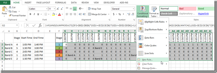 Then click on the Home Ribbon and then the Conditional Formatting Button and the New Rule menu item.
You will then see this pop up dialog box where you will need to click on the “Use a formula to determine which cells to format”
And then enter in the formula =g2=0 in the “Format values where this formula is true;” field and then click on the Format… button on the bottom right corner: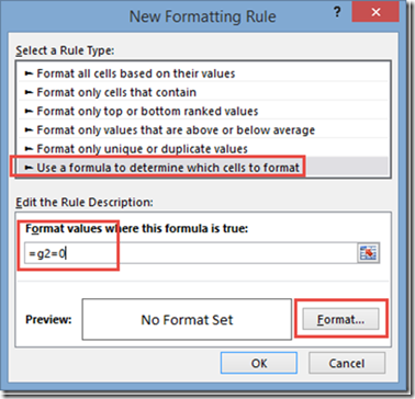
If you want to know more about the Tricks About Writing Conditional Formatting Rules, check out this post:
The Tricks to Writing a Conditional Formatting Rule Formula
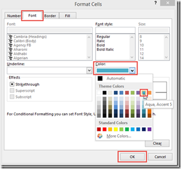
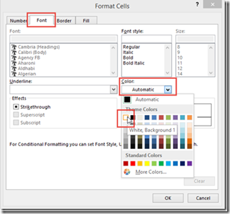
You will then see this pop-up dialog box and we want to change Font color from Automatic to White: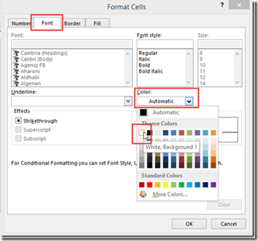
Then click on the OK button on both pop-up dialog boxes and you will then see that your formatting has taken effect and that the values that were previously showed as a Zero (0) are now appear to be blank.
5) Create Conditional Formatting for Right End of the Bar
To do this, once again, you will need to highlight the worksheet cells from cells G2:AI6. ![clip_image009[1] clip_image009[1]](https://www.exceldashboardtemplates.com/wp-content/uploads/2015/06/clip_image0091.png) Then click on the Home Ribbon and then the Conditional Formatting Button and the New Rule menu item.
Then click on the Home Ribbon and then the Conditional Formatting Button and the New Rule menu item.
You will then see the New Formatting Rule dialog box and you will want to to click on the “Use a formula to determine which cells to format”
Now in order to check if the cell is the right most of this band’s stage time, we need to check 2 things. One, is the cell to the right =0 and is the current cell <> 0. To do that, we enter in the formula =AND(OFFSET(G2,0,1,1,1)=0,G2<>0) in the “Format values where this formula is true;” field and then click on the Format… button on the bottom right corner: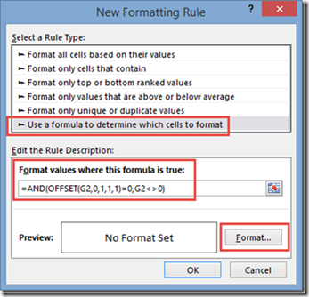
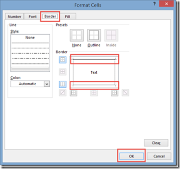
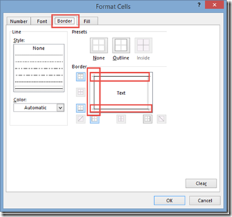
You then see this dialog box where we want to add a Right vertical Border: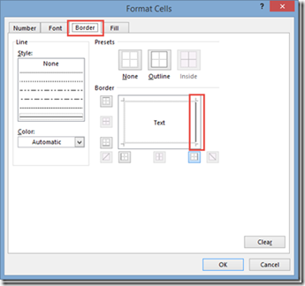
Then click on the OK button on both pop-up dialog boxes and you will then see that your formatting has taken effect and that the values that a vertical right border is now imposed on the cells where the band’s time on stage ends.
6) Create Conditional Formatting for Middle Bar Area
Follow all the same starting steps as above (i.e. Create a New Conditional Formatting Rule after you highlight the worksheet cells from cells G2:AI6.)
Then click on the “Use a formula to determine which cells to format”.
Now in order to check if the cell is in the middle of the band’s stage time, we need to check if the current cell = 1. For that, we enter in the formula =G2=1 in the “Format values where this formula is true;” field and then click on the Format… button on the bottom right corner:
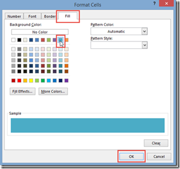
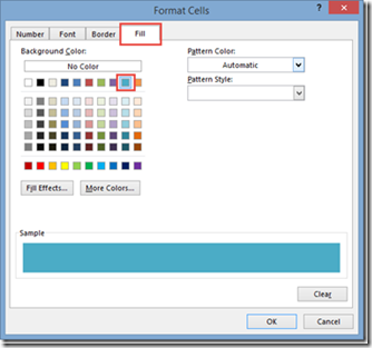
Then update your Font color to match the stage color, Add top and bottom borders and change the fill color to the same as the stage color.
After clicking on okay, you will then see the formatting has been applied to the middle bar areas like you see here:
7) Create Conditional Formatting for Left End of the Bar
This is the final time we need to do this, but once again, you will follow the same steps as above (i.e. Create a New Conditional Formatting Rule after you highlight the worksheet cells from cells G2:AI6.)
Then click on the “Use a formula to determine which cells to format”.
Now in order to check if the cell is the left end of the bar that also contains the the band name, we need to check if the current cell ISTEXT. For that, we enter in the formula =ISTEXT(G2) in the “Format values where this formula is true;” field and then click on the Format… button on the bottom right corner: 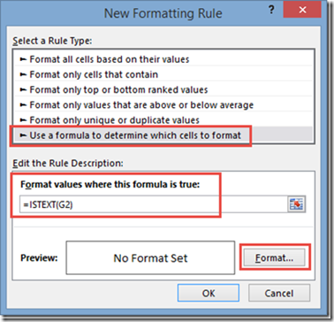
Then update your Font color to White, Add top, left and bottom borders and change the fill color to the same as the stage color.
Now your chart should now look like this: If you really want to get fancy, you can repeat the steps above and change the fill color to the stage colors to give it a little more definition. But in order to do this, you would repeat steps 4-7 for every row:
Notice how each color applies to a different range of just the stage row and not the entire stage chart area
Your new chart using that process would look like this: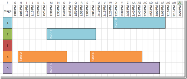
8) Adjust the Text Alignment to Vertical
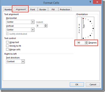
This is a step I like to do so that my stage times in Row 1 are about the same size. To do that, highlight cells G2:AI6 and click on the Alignment settings button to bring up the Alignment Options dialog box: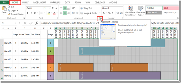 Then change the Alignment Degrees to 90 and press okay to make the band names display vertically as you see above.
Video Demonstration
Watch a video demonstration here:
Free Excel Conditional Chart Template Download
Download a free sample Excel file here:
Conditional Formatting Band Stage Chart.xlsx
I love conditional formatting and I wish you could do even more with it, but some things are just not an option in the Format Cells dialog box, but it can typically give you what you need. Do you like Conditional Formatting in Excel? Do you use it a lot? I find that I use it most for finding duplicates or specific values in a large data set. How about you? Let me know in the comments below.
Steve=True


