Easily Add Task Information to Excel 2016 Gantt Charts
Excel 2013 and Excel 2016 make this need so much easier. Thanks Excel! I recently posted a request from a fan that asked how to add task information to Excel 2016 Gantt Charts. With this technique, there is no need to do all the work of the previous post that we had to do for Excel 2007 and Excel 2010. Check out how we cut the steps in half below.
The Breakdown
The crux of this technique is to add another data series to the chart that will be put on the secondary axis so that the labels can display alternate categories.
1) Create Chart Data and Stacked Bar Chart
2) Modify Primary Axis
3) Add Chart Labels
4) Modify Series Fill Options
5) Chart Clean Up
Step-by-Step
1) Create Chart Data and Stacked Bar Chart
Assuming we start out with our data in this format:
| A | B | C | D | |
|---|---|---|---|---|
| 1 | Phase | Task | ||
| 2 | Duration Filler | Duration (Days) | ||
| 3 | Plan | Requirements | 2/5/2018 | 7 |
| 4 | Design | 2/12/2018 | 14 | |
| 5 | Develop | Development | 2/26/2018 | 63 |
| 6 | Unit Test | 4/30/2018 | 7 | |
| 7 | Deploy to QA | 5/7/2018 | 7 | |
| 8 | Test | UAT Test | 5/14/2018 | 21 |
| 9 | Bug Fix | 6/4/2018 | 7 | |
| 10 | Deploy | Deployment | 6/11/2018 | 7 |
| 11 | Training | 6/18/2018 | 14 |
First add 2 columns of data to your Excel Gantt Chart data range.
A) In column “E” add a series called “Resource Filler” to the right of the duration data. In Cell E3 enter a value of 100 for all cells so that we can see it easily in the chart. We will use this series for the labels and eventually, we will change this to a value of 0 so that it does not appear on the chart.
B) In column “F” add resource names for your labels by task line.
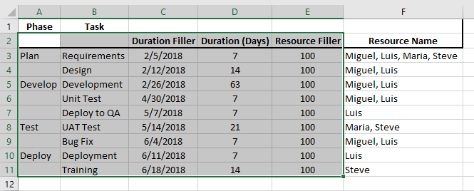
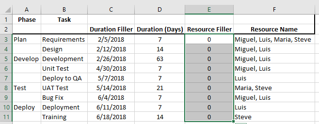
Your chart data should look like this:
| A | B | C | D | E | F | |
|---|---|---|---|---|---|---|
| 1 | Phase | Task | ||||
| 2 | Duration Filler | Duration (Days) | Resource Filler | Resource Name | ||
| 3 | Plan | Requirements | 2/5/2018 | 7 | 100 | Miguel, Luis, Maria, Steve |
| 4 | Design | 2/12/2018 | 14 | 100 | Miguel, Luis | |
| 5 | Develop | Development | 2/26/2018 | 63 | 100 | Miguel, Luis |
| 6 | Unit Test | 4/30/2018 | 7 | 100 | Miguel, Luis | |
| 7 | Deploy to QA | 5/7/2018 | 7 | 100 | Luis | |
| 8 | Test | UAT Test | 5/14/2018 | 21 | 100 | Maria, Steve |
| 9 | Bug Fix | 6/4/2018 | 7 | 100 | Miguel, Luis | |
| 10 | Deploy | Deployment | 6/11/2018 | 7 | 100 | Luis |
| 11 | Training | 6/18/2018 | 14 | 100 | Steve |
Next, create a Stacked Column Chart.
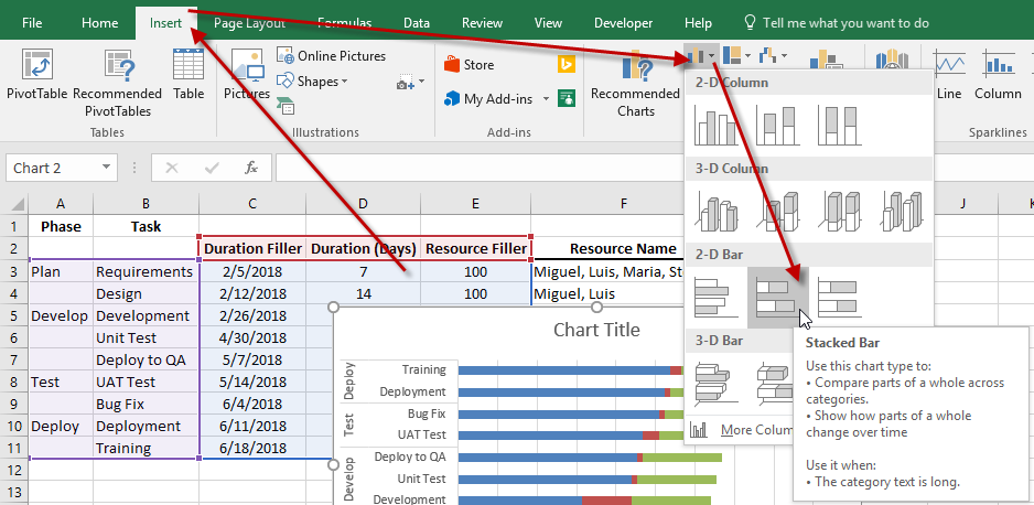
First highlight the chart data range A2:E11 as you see here:
Next, click on the Insert Ribbon and choose the Bar button in the Chart group and finally select Stacked Bar Chart as you see here:
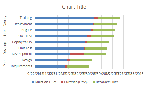
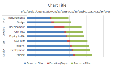
Your chart should now look like this:
2) Modify Primary Axes
Both the horizontal axis and the vertical axis have issues that should be corrected. For the vertical axis it should be reversed so that Plan is on top and Deploy on the bottom. For the horizontal axis, we should change the start date to a 2018 as our Excel Gantt Chart won’t span years prior and we should remove the year from the number format.
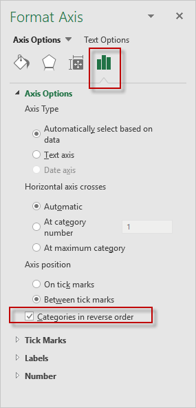
A) Reverse Vertical Axis Direction
Move the Plan phase to the top of the vertical axis by first selecting the chart. Then double click on the vertical axis or select it and press CTRL+1 and it will bring up the Format Axis dialog box. Finally, click on the “Categories in reverse order” checkbox under “Axis Options” and press the close button.
The chart should now look like this:
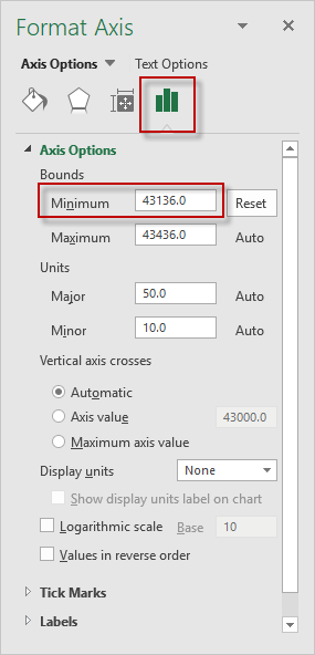
B) Set Horizontal Axis Minimum Value
To show a small task duration on our chart, you will need to set a fixed minimum bound value on the chart’s horizontal axis to a more recent date. It appears that Excel has changed it’s behavior from Excel 2010 where it set the minimum date to January 1st, 1900 to the a more reasonable date. In my sample data, the horizontal minimum bound is set to 43000 which is the nearest 1,000 value from our minimum date of 2/5/2018 which has a value of 43,316. As April 5, 2018, is our minimum value on the Duration Filler column and as a number that is equal to 43,136 (that many days since 1/1/1900), so it is best if we start are chart at that date.
To set your horizontal axis minimum, select the chart, then double-click on the horizontal axis to launch the Format Axis dialog box. Or, you can select the horizontal axis in the chart and press CTRL+1. Then change the minimum bound to a value of 43,136 as you see here:
Your chart should now look like this:
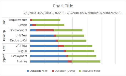
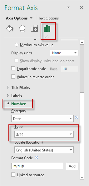
C) Change Horizontal Axis Number Format
After the change to the minimum bound value for the Horizontal Axis the dates are more readable, but some almost overlap. To fix this, we can modify the number format in the chart axis.
To change the number format on the horizontal axis, select the chart, then double click on the horizontal axis or you can select it and press CTRL+1. Either one will launch the Format Axis dialog box. Next, open the collapsed Number section and then select a Type of a short date like 3/14 to just show the day and month as you see here:
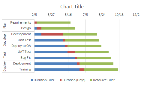
The chart should you have modified should now look like this with better dates on the Horizontal Axis:
3) Add Chart Labels
We can now Add Task Information to Excel 2016 Gantt Charts by adding labels to the “Resource Filler” chart series and then modify them to display values from cells instead of the value.
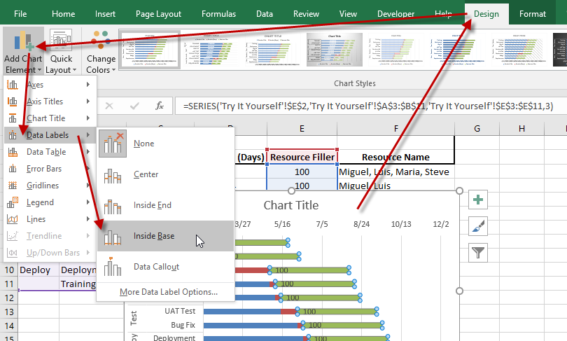
A) Add Outside End Chart Labels
First select the chart, then select the “Resource Filler” Chart Series then select the “Design” Ribbon, then choose “Add Chart Element” then “Data Labels” and then “Inside Base” option as you see here:
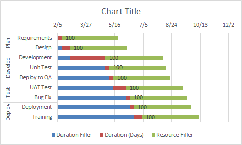
The Gantt chart with data labels should now look like this:
B) Change Data Labels to Categories
Excel 2016 default for data labels in a chart will display Values and we need to change ours to Value from a Cell.
To do that, select the chart, then double-click on any of the data labels “100” that you see in the Resource Filler bars or select any data label and press CTRL+1 to bring up the “Format Data Labels” dialog box.
Then “check” the “Value from Cell” checkbox and select the range on the worksheet from F3:F11. Then you need to remove the values when you “uncheck” the “Values” checkbox as you see here:
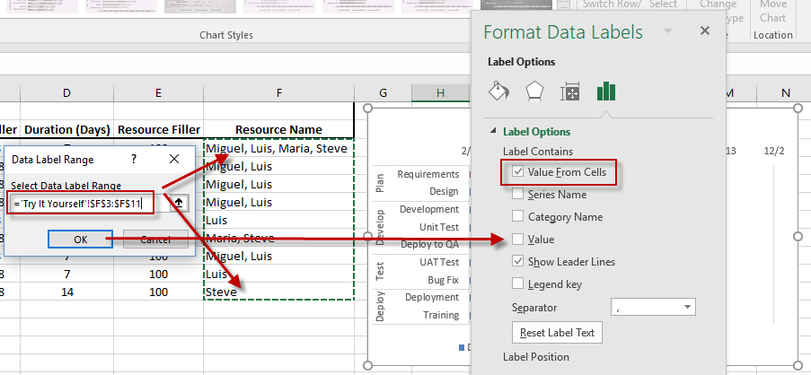
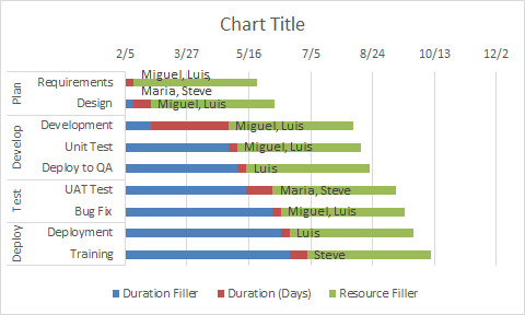
The chart will now have the Resource Names appearing as a data label:
4) Modify Series Fill Options
Our next step is to modify the “Duration Filler” series and “Resource Filler” fill colors. For the Excel Gantt Chart to have a Gantt Chart look, we need to make these series disappear on screen.
To do this, select the chart and then either double click on the “Duration Filler” series, or select the series and press CTRL+1 to bring up the Format Series dialog box. Then click on the Fill options and choose “No Fill” so that the series is now not visible but still there.
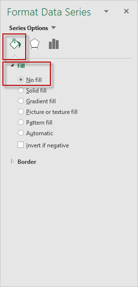
Repeat this step for the “Resource Filler” series by double clicking on the series in the chart or select the series and press CTRL+1 to bring up the Format Series dialog box. Then click on the Fill options and choose “No Fill” to hide it from view.
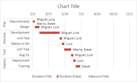
The chart should now look like this:
5) Chart Clean Up
The final step in most Excel 2016 Gantt Chart development is to clean up the chart of unneeded items.
A) Modify Resource Filler Value to Zero
Now that we have created our labels, there is no reason to show such a large value in the chart for the Resource Filler series. This is pretty simple, just update the values of 100 in the worksheet to zero so that this value doesn’t change the horizontal axis bounds.
B) Delete Chart Legend
First select your chart, then select the Legend and then press the delete key.
C) Delete Chart Title
Final step is to select your chart, then select the Title and then press the delete key.
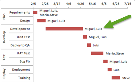
Your final Excel Gantt Chart with additional task information should now look like this:
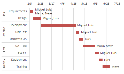
You can use this technique to show any task information in your Gantt charts that you wish, such as Percent Complete (% Complete), Assigned Resources, Start Date and Finish Date. The possibilities are only limited by your imagination.
Check Out Other Tutorials Related to this Article:
https://www.exceldashboardtemplates.com/FixMissingMulitLevelCategoryLabelOption
https://www.exceldashboardtemplates.com/GanttChart7EasySteps
Video Demonstration
Check out this Video tutorial on the techniques presented above.
Sample File Download
Click here to Download the Free Sample Excel Template File:
How-to-Add-Resource-Names-to-Excel-Gantt-Chart-Tasks-2016.xlsx
Your Thoughts and Comments
Excel 2013 and Excel 2016 makes it so much easier to do this than in previous versions of Excel. With this technique, you can use this trick to add more detail to any line chart, column chart or bar chart within Excel. Let me know your thoughts in the comments below.
Please make sure you sign up for the free newsletter so that you get the notification of the next article.
Steve=True


