A big shout out to Pete who submitted this answer to my last Friday Challenge.
You can check out the challenge here:
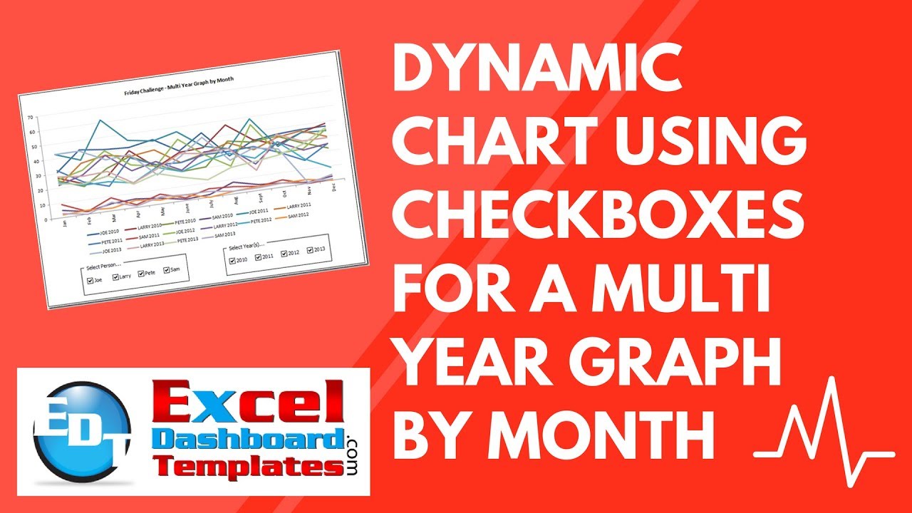
Friday-challenge-excel-mutli-year-graph-by-month

Check out the video and download the free Excel template file below.
Here is what Pete is doing:
1) Created Data Range linked to Check Boxes

2) Created Formulas to Show Data or #N/A based on Check Box Values

3) Created a Chart on the Formula Data

4) Created a Macro to hide rows (thus hiding the chart lines) when a #N/A is Present.
(Pete, let me know if I got it wrong ![]() )
)
Check it out by checking the check boxes in the file below.
File Download:
Petes-Friday-Challenge-Mutli-year-Graph-by-Month-Solution.xlsm
Video Demonstration:
Thanks for an inventive solution Pete.
Steve=True


