Hands off to Leonid 🙂 for this awesome solution with much Much BETTER formulas for a recent Friday Challenge.
Here was the original Challenge:
friday-challenge-pipeline-usage-chart
Here was my solution that this post references:
pipeline-challenge-matching-stacked-bar-chart-colors-to-products-without-vba
Leonid modified the 2 formulas that I used in my Area Chart solution, but he did it much more efficiently. And I learned a lot from how he create his formulas and you may as well. Here is Leonid’s description of how his formulas work.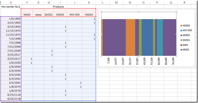
Horizontal Axis Categories Formula (Dates on the left most column of the picture above):
Here was the original formula from my solution:
=IFERROR(SMALL(Table1[Cumulative Pipeline (Leave as Date)],TRUNC(ROW(A1)/2,0)),IF(ISBLANK(E2),0,IF(E1=E2,””,E2)))
Instead Leonid Created this Formula:
=IFERROR(SMALL(MMULT($C$3:$C$14,{1,1}),ROWS($A$1:A1)),””)
Here is how Leonid’s formula works:
MMULT function is designed to return the result of matrix multiplication of two arrays.
The result is an array with number of rows in array1 and number of columns as in array2.
In this example MMULT($C$3:$C$14,{1,1}) returns 12×2 array e.g.
{0,0;1179,1179;25887,25887;35979,35979;40025,40025;42819,42819;54828,54828;57042,57042;59234,59234;65388,65388;79800,79800;20566,20566}
It is a two columns array with a duplicated set of values from $C$3:$C$14 – exactly what we need for our Step chart.
And when we pass it to the SMALL function along with the sequential numbers generator ROWS($A$1:A1) we got ordered values one at a time pair after pair.
It works OK if we do not have blanks in $C$3:$C$14.
By nature of the Step chart we shouldn’t have gaps there, but if we populate only e.g. C3:C9 with values and reserve the rest of cells for the future entries, we’ll need to define a dynamic range and instead of C3:C14 use something like $C$3:INDEX(C:C,COUNT(C:C)+ROW($C$2),)
Then the resulting formula will be
=IFERROR(SMALL(MMULT($C$3:INDEX(C:C,COUNT(C:C)+ROW($C$2),),{1,1}),ROWS($A$1:A1)),””)
We do need IFERROR in case we copy the formula down one or more rows farther than we need for the chart.
Values by Product Formula (“1” or Blanks in the data area below the Product names):
Here was the original formula from my solution (non-Array Formula):
=IF($E3=0,IF(INDEX(Table1[Product Name],MATCH($E4,Table1[Cumulative Pipeline (Leave as Date)],0))=F$2,1,””),IFERROR(IF(AND(F2=1,F1=1),””,IF(SUM($F1:$K2)=2,IF(IFERROR(INDEX(Table1[Product Name],MATCH($E4,Table1[Cumulative Pipeline (Leave as Date)],0))=F$2,FALSE),1,””),IF(IFERROR(INDEX(Table1[Product Name],MATCH($E3,Table1[Cumulative Pipeline (Leave as Date)],0))=F$2,FALSE),1,””))),IF(INDEX(Table1[Product Name],MATCH($E4,Table1[Cumulative Pipeline (Leave as Date)],0))=F$2,1,””)))
Instead Leonid Created this Array Formula:
{=IF(OR(($F4=Table13[Cumulative Pipeline (Leave as Date)])*(G$2=Table13[Product Name])),1,””)}
NOTE: Curly brackets are not entered but appear when you press CTRL+SHIFT+ENTER when completing the formula to make it an array.
The array formula
=IF(OR(($F4=Table13[Cumulative Pipeline (Leave as Date)])*(G$2=Table13[Product Name])),1,””)
for the data area is a two way lookup that tells us if there is any match in in the source records where the product is the same as the header of the current column and the date is the same as the date in the next row.
In case of true we flag it with 1 and set to empty string if it’s not.
The product of two Boolean arrays will produce an array of 0s or 0s and 1s.
OR function tells us if there is any 1 there.
SUMPRODUCT also will work and might be even better, because then the formula doesn’t have to be array entered:
Example of SumProduct formula =IF(SUMPRODUCT(($F4=Table13[Cumulative Pipeline (Leave as Date)])*(G$2=Table13[Product Name])),1,””)
File Download
Here is the free sample file download with Leonid’s formulas in action:
Pipeline-Usage-Chart-without-VBA-Leonid.xlsx
If you want to see how Pete solved this with VBA, check out this post:
match-product-chart-colors-to-excel-spreadsheet-cells-petes-vba-solution
THANKS again Leonid! What a cool solution. I definitely need to learn more about arrays, but I definitely learned more about the MMULT function. Thanks for sharing this with us.
Steve=True


