Here is the first and easiest answer to the challenge on posted on Friday.
In case you missed it, you can check it out and download the sample data file here:
So far, we have had several answers and none were the same. However, the absolute easiest is this manual process submitted by Don.
The Breakdown
1) Copy and Paste Entire Data Range
2) Delete First Date Data Point and Shift Cells Up
3) Delete Last Rate Data Point of Original Data Area and Shift Cells Up
4) Create Line Chart
Step-by-Step
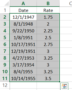
1) Copy and Paste Entire Data Range
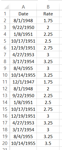
| Date | Rate |
| 12/1/1947 | 1.75 |
| 8/1/1948 | 2 |
| 9/22/1950 | 2.25 |
| 1/8/1951 | 2.5 |
| 10/17/1951 | 2.75 |
| 12/19/1951 | 3 |
| 4/27/1953 | 3.25 |
| 3/17/1954 | 3 |
| 8/4/1955 | 3.25 |
| 10/14/1955 | 3.5 |
Highlight your data range and copy all data.
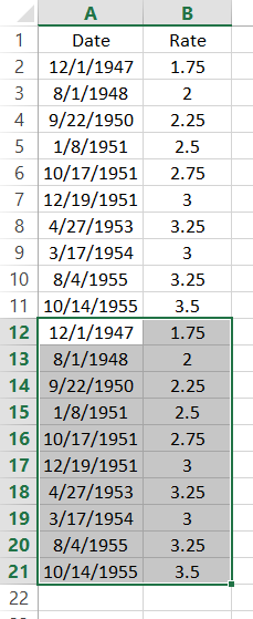
Then paste the data below the original data set.
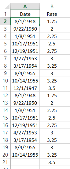
2) Delete First Date Data Point and Shift Cells Up
Now select the first date value in column A
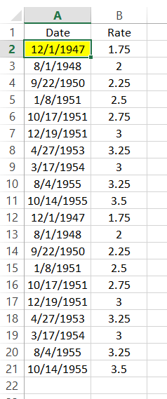
and select the delete cells menu option from the Delete Button on the Home Ribbon.
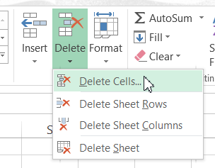
Choose to shift cells up.
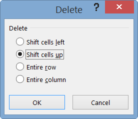
Your new chart data range will now look like this:
3) Delete Last Rate Data Point of Original Data Area and Shift Cells Up
Now select the last rate data point in column B
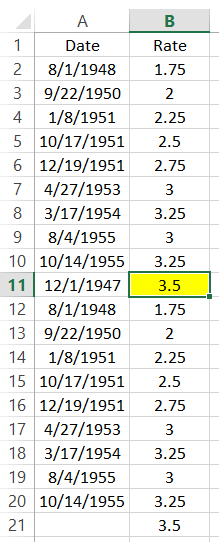
and follow the same delete steps as shown above to shift the cells up. Your new chart data range will now look like this:
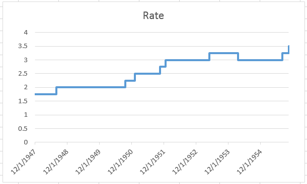
4) Create Line Chart
Now that we have our new data set, you can create your line chart by simply highlighting the chart data range and creating a line chart.
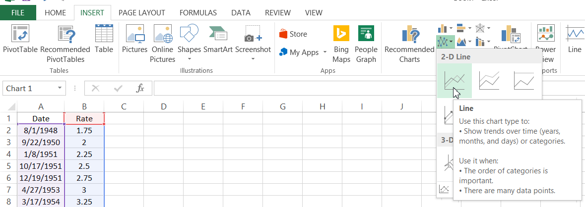
Your new Excel Step Chart should now look like this:
Video Tutorial
Check out this quick video here:

Thanks Don! Great solution.
Steve=True


