Friday Challenge Solution – Excel 2013 Data Labels on a Range

In our last Friday Challenge,

we were trying to help Kevin with his problem.

He had followed this tutorial to add more lines to his Excel Chart Data Table:

And he wanted to add one more line to his Data Table but Excel would only let him put in numbers or values and not text.

Kevin wanted to put in if the column of data was related to a part or an assembly.

Here is Don’s solution. Mind you, this only works for Excel 2013.

Don suggests that Kevin put in Data Labels in the chart and then link those values to the Part/ASM column.

First, create your chart, then add data labels to the chart.

Then select the data labels and press CTRL+1 to bring up the data label options.

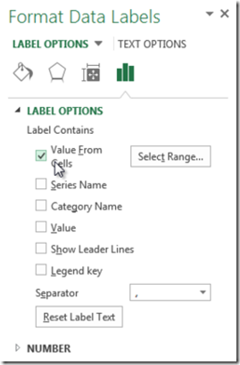
In 2013, you will now see this new label option under Label Contains called “Values from Cells”.

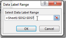
Check that box and then click on “Select Range…”

and choose the Part/ASM data in your Excel Spreadsheet:

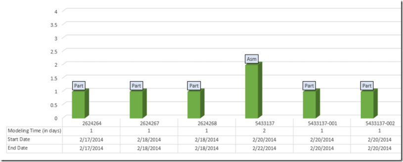
then your labels will now be linked to those cells. What a great change to the Excel 2013 edition. Your chart will now look like this:

Here is a video tutorial showing you how this works in Excel 2013:

Thanks Don! This is a very simple solution and I think it does the trick.

Come back tomorrow to see additional solutions for this challenge.

Steve=True

Stay Connected!