Here is how you can quickly solve the most recent Friday Challenge: Find Unique Values from CSV List
Before we begin, I am going to show you how to do this with some standard Excel features and functionality. Now one way that you can solve this that I won’t be showing you today is to use PowerQuery in Excel. If you have a lot of these types of questions coming up in your daily life, I would highly recommend that you visit some PowerQuery posts to learn more.
Now onto my tips and tricks to solving this problem.
Problem Recap
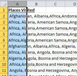
The marketing department posted a survey on your companies website and they need to find the Top 3 countries visited by survey respondents. HOWEVER, the website developer didn’t understand and the answers came back as a list by each user in one text string of values separated by commas.
Can you Find Unique Values from CSV List, put your answers in the comments below.
- Top 3 Countries Visited
- Total Number of Countries Visited.
- Bonus Question = How many total country visits were identified in this sample data
The Breakdown
1) Convert Data from 1 Column to Many
2) Add Column and Row of ID Numbers
3) Convert Data to Pivot Table
4) Explode Data Set from Pivot Table
5) Remove Extra Spaces
6) Create Country Visits Pivot Table
Step-by-Step
1) Convert Data from 1 Column to Many
To do this, select Column A of the data:
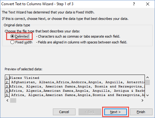
and then go to the Data Ribbon and press the Text to Columns Button

Choose the Delimited checkbox and then select the next button.
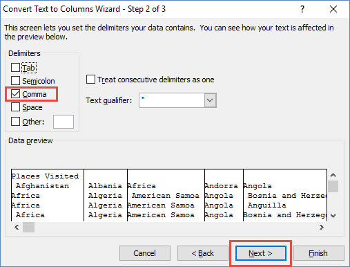
Choose the Comma checkbox and then select the next button.
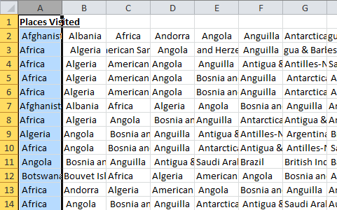
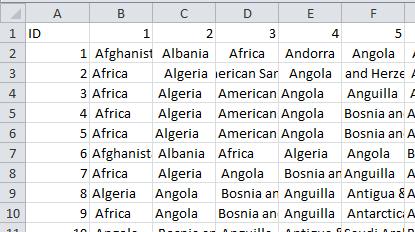
Your data will now look like this:
2) Add Column and Row of ID Numbers
This is a pretty easy step that most people can do 🙂 just insert a column to the left of column A by right clicking on column A and selecting the Insert Pop-up Menu Option.
Then create ID numbers in the first 2 rows and or columns and use the fill handle to create a unique ID for each row and column.
Your spreadsheet will now look like this:
3) Convert Data to Pivot Table
Now that our data is setup we can make Excel create a Pivot table of this data even though it is in a non-standard data table. To do that, you need to use an old Excel Wizard that you can only launch with the following key strokes:
On your keyboard press ALT+D and then press P.
Update: If you are using Excel in a different language, you may need to find the correct way to open this dialog box. Note this comment for Dutch from Akke: “I had to find out the Dutch (ALT A, A, D) shortcut to the old pivot tables. Met vriendelijke groet, with kind regards”
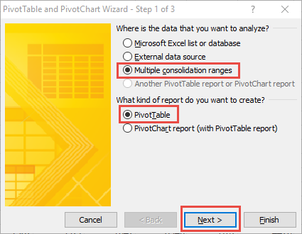
This will bring up the legacy pivot table wizard from Excel 2003.
Next, select Multiple Consolidated Ranges and press the Next button:
Then in step 2a of the wizard, leave the “Create a Single Page Field for Me” selected and press the Next Button:

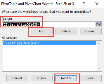
Then in step 2b of the wizard, click in the Range field and highlight your range on the spreadsheet. Then click on the Add button and then click on the Next button.
Final step 3 is to select New Worksheet to place the pivot table and then click on the Finish button:

Your pivot table will look like this:
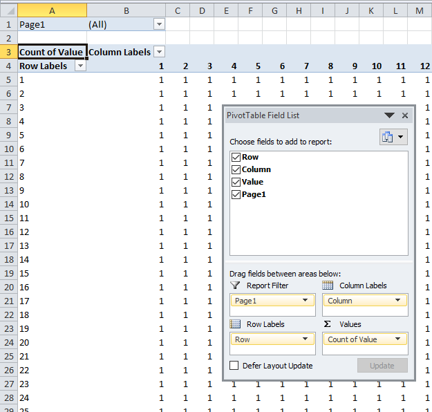
4) Explode Data Set from Pivot Table
Next get our data back into one column of data for every location visited, we need to explode the data from the newly created pivot table into a table of the data. To do this, find the Grand Total on the bottom right of the new pivot table and double click on it.
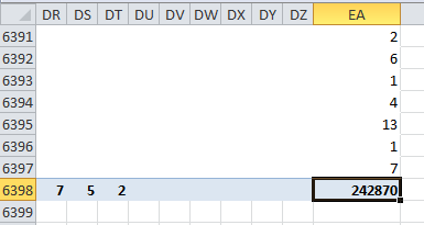
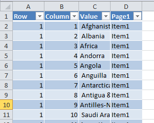
After doing so, your data table will look like this with all the values of the original CSV file in one data column.
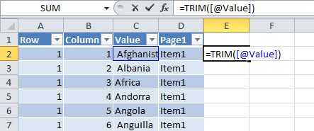
5) Remove Extra Spaces
Unfortunately, the new data still has leading spaces so there are duplicates that show up that are not really duplicates. To remove these, go to Cell E2 and put in a TRIM formula on cell C2. When you hit enter, it will fill in for the whole column as the pivot data is in an Excel Table.
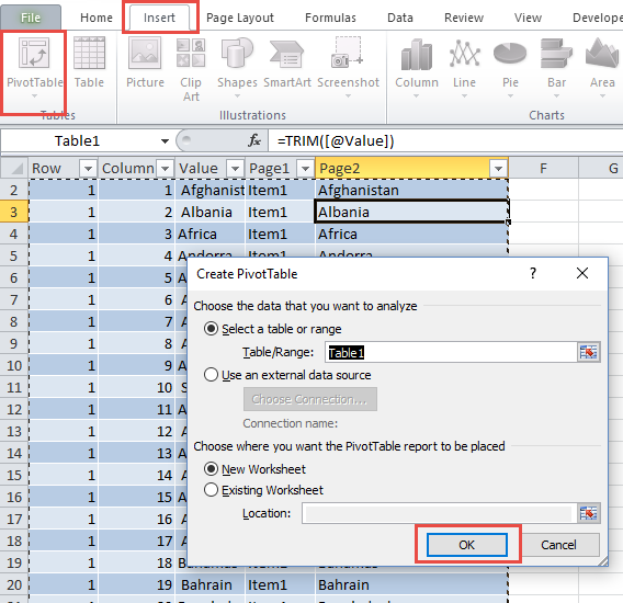
6) Create Country Visits Pivot Table
We finally have all the data we need. Final few steps are to:
a) Create a pivot table by clicking anywhere in the data table and then select the Insert ribbon and then select the Pivot Table Button and choose
b) Drag and Drop “Page 2” to the Rows and Values
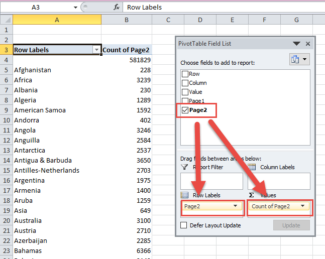
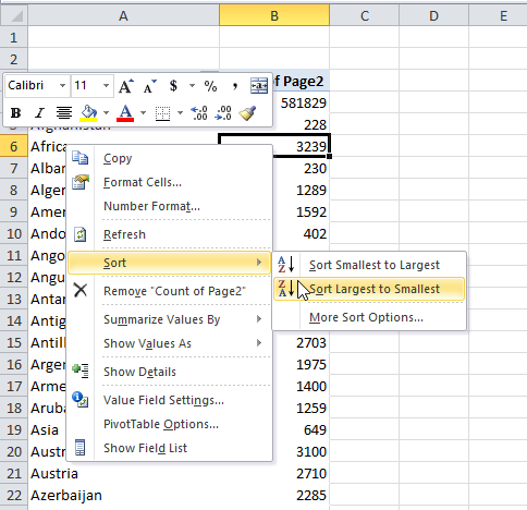
c) Sort Values Large to Small
Your Challenge Answer:
1- Bahamas / Cambodia / French Guiana
2- 181 (or 180 without Africa)
3- 242 868 (239 629 -Africa)
Here are other examples of this technique in action:
the-best-way-to-separate-address-text-to-multiple-columns
how-to-convert-an-existing-excel-data-set-to-a-pivot-table-format
Friday Challenge – Find Unique Class List in Excel ANSWER
Video Demonstration
Check out the video tutorial for this Excel Tip/Excel Trick to Find Unique Values from CSV List:
Let me know if you like this method or prefer PowerQuery in the comments below.
Steve=True


