On Friday, I posted this challenge:
You can download the sample data set here: Challenge Sample Data
Check out the post and download / try it yourself before you read this post.
Challenge Data Creation
Well, good news is that I know the answer because I created the data.
- I went to a local university and found their class list
- I randomly added a space to the beginning and the end of some of the classes and added those to the original list (I did this because like the project, several of the entries were the same, except for extra spaces)
- I added a few extra entries to the list of bad data like #, $, % etc.
- I then randomly added the data to multiple columns and rows using choose, randombetween and vlookup
Challenge Answer
1. Add a column of data to the original data as a row counter.
This is a simple step, just insert a column before Col1 and then add text “Row 1” in A2 and “Row 2” in A3. Then copy this down to the end of the data set. We do this because we want a unique identifier for all the data instead of the first column of actual data. You should have 2000 rows of data in the Excel Spreadsheet.
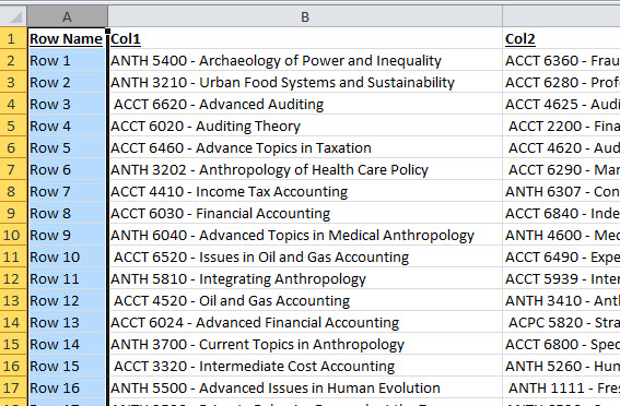
2. Use Multiple Consolidated Ranges to Create Pivot Table of the original data
This step will take all the data and puts it into a pivot count. We will then use this Pivot Table to get all the columns of data into one column of data.
How-to Convert an Existing Excel Data Set to a Pivot Table Format
Your new Pivot Table will now look like this with a grand total of 69,650 data points.
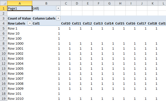
3. Explode Data from Newly Created
By double clicking on the Grand Grand Total, your newly created Pivot Table will take all of the data out of the original format and put it into one single column. Double click on the Grand Grand Total to explode the data into a new worksheet tab that will show you each unique entry. It should be in cell AZ2005 and have a value of 69,650.
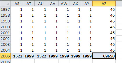
Your data will now look like this:

4. Trim Data to Remove Spaces
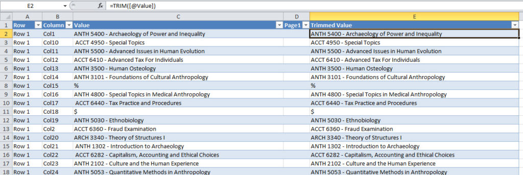
I always suggest that you remove all spaces and see if there is duplicate data. In case of this project, there were leading and trailing spaces. This mean that our count would not be correct and we would then send the wrong data to our client that included duplicates. So always trim the data if you can remember.
On the new worksheet tab with the exploded data from the consolidated Pivot Table. First add a header title of “Trimmed Value”. Then in cell E2, we need to add a new formula in the column =TRIM([@Value]). The Excel Table will take over and copy this formula down the column.
5. Create new Pivot Table from Exploded Data
Only one step left. With your new Trimmed Space class list data, we will create a new Pivot Table to count all the unique values. Just click anywhere in the data and then go to your Insert Ribbon and click on the Pivot Table button. Add the Trimmed Value to the Row Labels and Values.
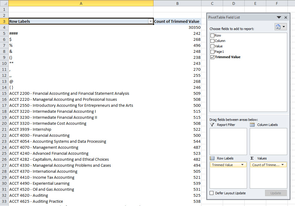
You will notice that there are 30,350 values that are blank. In order to check that our data matches the original, you should remove the check mark next to the Blank from the Row Labels Down Arrow (Row Labels Picklist).
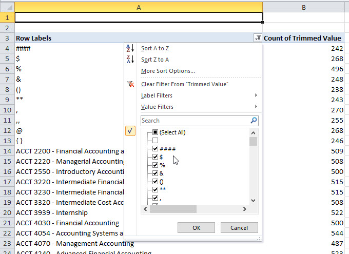
If we do that, we see that there at 69,650 values. That matches our original data as seen in the original Multiple Consolidated Range Pivot Table as well as just highlighting the data only in the Original Data tab. So we have the right count of data points and are not double counting any data or missing any data.
Now to find the final answer, we also want to filter out the values in the Pivot Table for the Row Labels to and uncheck the code/characters of ####, $, %, &, (), **, ‘,’, “, @, and {}. Then you will get the final count and answer you seek.
The final count of unique class values in our data set is…..
186
Is this the same technique that you used? One of the participants of the challenge used Get and Transform from the new Excel 2016 version. Did you use a formula? Let me know in the comments below!
Video Demonstration
Here is a video tutorial of the technique described above.
Thanks to everyone that submitted answers to the challenge!
Steve=True


