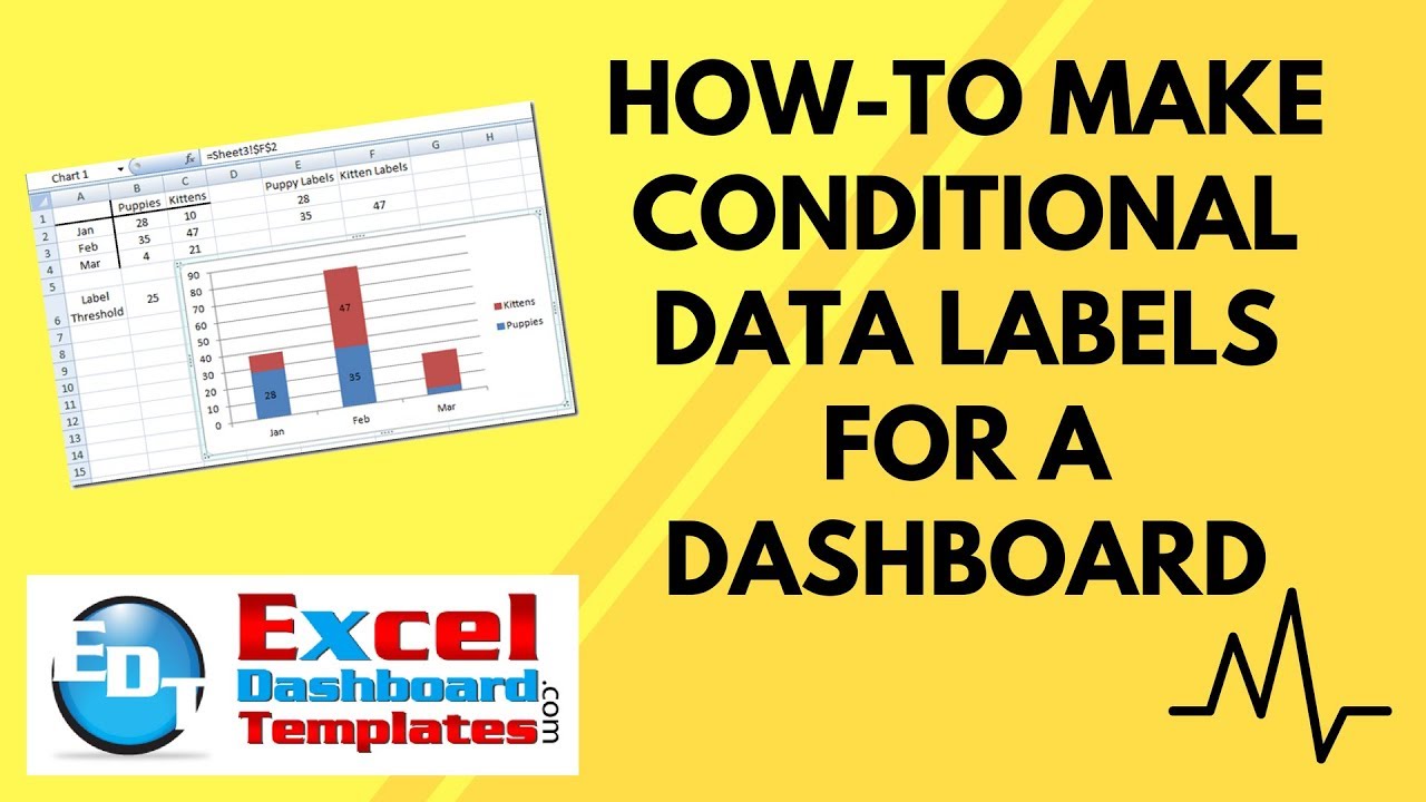
Recently I was thinking that sometimes when you make a Stacked Column Chart in your Excel Dashboard, you may want to hide some of the smaller values. This is especially true when some of the values are really small and the chart data labels may overlap. For example, in this chart you see that we are not showing a value for Kittens in January and also not showing a value for Puppies in March.

So it got me thinking about how we can do this in Excel. I also thought, how can we make a the labels conditional based on a value that I enter in the spreadsheet?
And I came up with this solution…
Breakdown
1) Create a New Conditional Data Label Range
2) Create Chart and Add Data Labels
3) Change Data Labels to the New Conditional Data Label Range
Step-by-Step
1) After you create your Chart Data Range, you now need to create the conditional labels data range. Given my example below, I have put the chart data in cells A1:C4 and then I put this formula in cell
E2 =IF(B2>=$B$6,B2,””)
Then copy this formula down and over into cells E2:F4
Then put your Conditional Label Threshold in Cell B6. In this case, I used 25.

2) Create your chart by highlighting cells A1:C4. Then go to the Insert Ribbon and Chose the Conditional Stacked Column Chart.

3) Select the chart and then insert data labels by going to the Layout Ribbon and choosing Data Labels from the Labels group.

Then select each individual data label by clicking on each label 2 times. Once you have selected each individual data label, press the “=” (equals sign) and then select the corresponding New Data Label that you created in cells E2:F4.
Repeat this process for each of the individual data labels in the Excel Dashboard Chart.
Now each of the data labels that are greater or equal then your Label Threshold (cell B6) will now conditionally appear in the chart as you change the threshold.
See a detailed video tutorial below. Also, please check out this additional demonstration of how to make your own custom data labels.
How-to Add Custom Labels that Dynamically Change in Excel Charts
Video Tutorial:
Please leave me a comment and let me know what you think of this post. Also, please sign up for the blog RSS feed so you get the latest post.
Steve=True


