As an Excel dashboard engineer you will often need to create complex calculations for your charts, tables and displays. So today’s challenge is one that was sent in by a reader from another of my posts.
Excel-formulas-average-a-range-and-ignore-zeros-0-value
“Hi really need your help, I would like to know how I can average different cells in different columns and ignoring zeros. For e.g take columns a to k, a will have an average that i need then c will have an average that i need and then e etc. The other columns will have other figures which I do not need. Please help i have used the following but did not help, =AverageIF(c3,e3,g3,i3,k3,”>0″) I have tried messing about with this but not sure where I am going wrong your help will be appreciated, many thanks in advance” – Shane
It seems like an easy solution, but the trick is that we need to calculate this averageif on non-adjacent columns of data. So I have set up some data for us for this challenge and it looks like this:
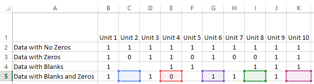
Can you figure it out? Leave a comment with your solution for cell N2 and it should work for all the rows with zeros, blanks and both zeros and blanks:
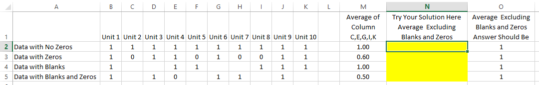
Here is the challenge data file for download: Challenge-Data-Average-Excluding-Zeros-and-Blanks-for-Non-Adjacent-Columns.xlsx
Good luck and thanks for playing the home game!
Steve=True
add a row K to put an X identifying which columns (c,e,g,i,k) to average and then use this formula
=AVERAGEIFS($B5:$K5,$B$6:$K$6,”X”,$B5:$K5,””””,$B5:$K5,”0″)
Thanks Ken. However, I think you may have meant Row 6 instead of K. Also, should the criteria be >0 instead of “0”? However, when I implement that, I am getting a #Div/0 error. Steve=True
Thanks again Ken, when I retype the formula, it seems to work for me. Not sure why the copy/paste isn’t. Also, you may not need the $b5:$k5, “””” criteria range and criteria as Excel appears to not include the blanks anyway. Thanks again. Steve=True
Hi Steve
This works for me:
=AVERAGEIFS(B5:K5,$B$6:$K$6,”X”,B5:K5,””,B5:K5,”>0″)
Thanks Xlarium, for some reason when I copy and paste, then redo the ” (quotes), I keep getting a #Div/0 error. When I typed it fresh, it worked. One thing, I don’t think you need the B5:K5,”” criteria range and criteria as Excel already ignores blanks in the Average If. Thanks again! Steve=True
=AVERAGEIF(C6:C6:E6:E6:G6:G6:I6:I6:K6:K6,”>0″)
I believe this works!
Nice one Laura, it worked for me as well. Great job. Steve=True
Hi Laura, as I investigated this solution further, it appears that Excel converts your range to the entire range and therefore, it doesn’t work for what we need here. For instance, if you change one of the numbers in cell B6 which should not be in the non-contiguous range, it will get calculated into the average.
I took from Ken’s idea and cleaned it up a little. Still have the add the “X” to row 6 though. =AVERAGEIFS(B2:K2,$B$6:$K$6,”X”,B2:K2,”0″)
Cool!
=SUM(B2:K2)/(COUNTA(B2:K2)-COUNTIF(B2:K2,0))
Thanks ME – Unfortunately, this one doesn’t seem to work over the non-contiguous range. If you put a value in the D column, it gets calculated in your formula. Thanks for trying. Steve=True
Maybe a bit complicated, but without any additional row:
=SUMPRODUCT((MOD(COLUMN(C2:K2),2)=1)*(LEN(C2:K2)>0)*(C2:K20)*(C2:K2))/SUMPRODUCT((MOD(COLUMN(C2:K2),2)=1)*(LEN(C2:K2)>0)*(C2:K20))
Thanks Pepe.