Today I have 2 formula challenges that you may find interesting. They are both different types of allocation formulas.
Challenge 1:
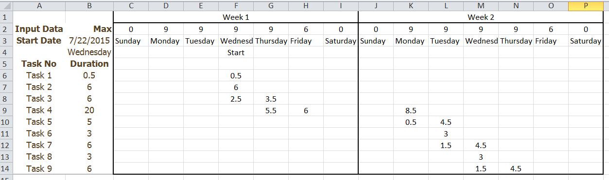
Problem: You have 9 tasks that each take a different amount of time to complete. The project will be completed over 2 weeks and it can start on any day of the week. Each day of the week has a maximum work time. Tasks can be started on one day and finish on another.
Challenge: Write 3 formulas:
1) Formula 1 in Cell B4 that displays the weekday name of the date entered in Cell B3.
2) Formula 2 for the start of the project that you can copy across the range C4:I4. Formula starts in Cell C4 and displays the word Start if the day of the week = start date of the project.
3) Formula 3 for the allocation of hours by task by day for the 2 week time period. Hours for the day cannot exceed the max hours for the day in row 2. Tasks can be started on one day and finish on another. If there is time left in the day, then the next task should be started.
Here is the data file: Allocation Challenge 1
This is what the final layout will look like if you are successful:
Challenge 2:
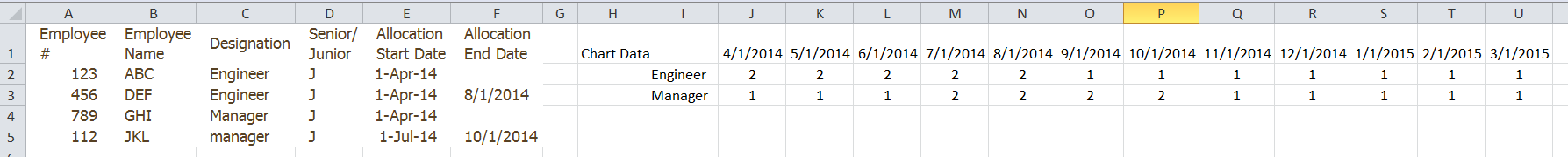
Problem: You have multiple allocations that you need to hire for over several months. You don’t want to have too many hires sitting on the bench, so you want to know how many you need in a given month. Allocations may be open ended or may have an end date. There are 2 types of designations of hires – Managers and Engineers.
Challenge: Write 1 formulas:
1) Formula 1 for the count of resource types that you need for a given month that can be copied across the range J2:U2.
Here is the data file: Allocation Challenge 2
This is what the final layout will look like if you are successful:
PS: Please put your formulas in the comments below.
Steve=True
Have not tried everything yet but my suggestion s far is for challenge 1:
Formula 1: =TEXT(WEEKDAY(DATE(YEAR($B$3);MONTH($B$3);DAY($B$3));1);”dddd”)
Formula 2: =IF(C3=$B$4;”Start”;””)
Fairly simple but works 🙂
/T
Thanks TJ! Your formulas work great.
Formula 1 can be greatly streamlined. You were very close. Just replace your weekday formula with B3
Formula 2 was an exact match 🙂
By the way, I had to substitute commas for semicolons. Do you have a semicolon set up as the default for your Excel version?
Steve=True
Hi
I will try with your feedback. Thanks.
Yes, I have ; set up as it seems. Nothing I have done on purpose. Could be that I reside in Sweden and we have different regional setups.
/T
Challenge 1
Formula 1:=LOOKUP(WEEKDAY(B3),{1,2,3,4,5,6,7},{“Sunday”,”Monday”,”Tuesday”,”Wednesday”,”Thursday”,”Friday”,”Saturday”})
Formula 2: =IF(COLUMN()>Start_col,MIN(F$2-SUM(F$5:F5),$B6-SUM($C6:E6)),IF(COLUMN()<Start_col,0,IF(SUM(F$5:F5)+$B6<=F$2,$B6,F$2-SUM(F$5:F5))))
Start_col is a named formula:=MATCH(Data!$B$4,Data!$C$3:$I$3)+2
Challenge 2
=SUMPRODUCT(–($C$2:$C$5=$I2),–($E$2:$E$5=J$1))
I put in dates for open end dates which were far in the future (ie 8/1/2100). Whey make it difficult if you don’t have to?
Challenge 2 did not show correctly in first comment:
Challenge 2
=SUMPRODUCT(–($C$2:$C$5=$I2),–($E$2:$E$5=J$1))
I put in dates for ending dates for open end which were far in the future (ie 8/1/2100).
When I type in the challenge 2 formula, the last part will not show up on the comment
=SUMPRODUCT(–($C$2:$C$5=$I2),–($E$2:$E$5=J$1))
Super old post, don’t care this was fun. Someone sent it to me, and it wa too fun
Challenge 1, Formula 1 in B4: =TEXT(B3,”dddd”)
Challenge 1, Formula 2 in C4: =IF($B$4=C3,”Start”,””)
Challenge 1, Formula 3 in C6: =IF(AND(COUNTIF($C$4:C$4,”Start”)>=1,SUM(C$5:C5)<C$2,(SUM($B6:B6)-$B6)<$B6),MIN($B6,2*$B6-SUM($B6:B6),C$2-SUM(C$5:C5)),"")
Challenge 2, Formula 1 in J2: =COUNTIFS($C:$C,$I2,$E:$E,"=”&J$1)+COUNTIFS($C:$C,$I2,$E:$E,”<="&J$1,$F:$F,"")
Thanks for the solution. Glad you had fun!