Excel Formula Formatting Quick Tip

Learn the best Excel Formula Formatting technique so that you can quickly edit them in the future! You will use these simple techniques for all of your Excel Formulas going forward.

Lately, I have been writing some very long and convoluted formulas in Excel.  Most developers have tools that show them their formulas in a better format.  And you too can do something similar in Excel.  Here is an alternate way to format your formulas for easy reading.

The Breakdown

1) Expand the Formula Bar

2) Enter Hard Returns as Desired

3) Enter Spaces as Desired

Step-by-Step

1) Expand the Formula Bar

If you didn’t know, you can make your formula bar larger to see more of the formula.

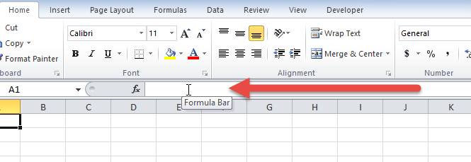
What is the formula bar?

The formula bar is where you see any entry that you have made in a particular cell within an Excel worksheet as you see here.

How do you expand it?

There are 3 ways that you can expand the visible area of your Formula Bar in an Excel worksheet.

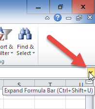
1) Click on the Expand Formula Bar control on the far right of the Formula bar as you see her:

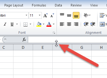
2) Manually expand the Formula Bar with the Formula Bar selector.

To do this, place your cursor in-between the Formula Bar and the Row Letter Indicators as you see here.

3) Adjust the size of the Name Box control.

If you absolutely need more space you can shrink the size of the Name Box and that will give you more visible space for your Formula Bar.  To shrink or resize the Name Box area, place your cursor on the far right of the Name Box and then click and drag as you see here.

2) Enter Hard Returns as Desired

Now that you can see more of your Formula Bar we can change our Excel Formula Formatting.

The trick is to use Hard Returns within your formulas by pressing ALT+Enter keys. You can learn more about the technique here:

Excel Line Break/Hard Return within a Cell

You should consider using the Hard Returns after logical sections.  For instance, you may want to use them as breakpoints for the True or False sections in a IF Function.  Another use case is to break up anything that can have multiple entries, like the AND Function, OR Function, or the CHOOSE Function.

Note, i think this should be combined with the next step, but here is a sample of how a formula would look with just hard returns added.

Before:

=IF(LEN([@Coordinates])=0, “”,IF(Display=”Line and Pin”,VALUE(MID([@Coordinates],FIND(“,”,[@Coordinates])+2,LEN([@Coordinates])-FIND(“,”,[@Coordinates])-2)),NA()))

After:

=IF(LEN([@Coordinates])=0,

“”,

IF(Display=”Line and Pin”,

VALUE(MID([@Coordinates],FIND(“,”,[@Coordinates])+2,LEN([@Coordinates])-FIND(“,”,[@Coordinates])-2)),

NA()))

You can more clearly see each breakdown of each of the IF Functions.

3) Enter Spaces as Desired

The final trick is to add “spaces” to enhance your Excel Formula Formatting in conjunction with the Hard Returns you put in above.  This will show a stepped or tiered effect on your formulas for ease of readability.

Here is what a complex formula looks like before and after

Before:

=IF(OR(HighlightCategory=”None”,HighlightCategory=”Right”),IF(LEN([@[Base Category]])>0,[@[Base Category]],”Add or Delete Base Category”),IF(LEN([@[Base Category]])<=1,””,CHOOSE(HighlightChoice,IF([@[Base Category]]<HighlightValue,[@[Base Category]]&” “&HighlightCategoryText,[@[Base Category]]),IF([@[Base Category]]>HighlightValue,[@[Base Category]]&” “&HighlightCategoryText,[@[Base Category]]),IF([@[Base Category]]<=HighlightValue,[@[Base Category]]&” “&HighlightCategoryText,[@[Base Category]]),IF([@[Base Category]]>=HighlightValue,[@[Base Category]]&” “&HighlightCategoryText,[@[Base Category]]))))

After:

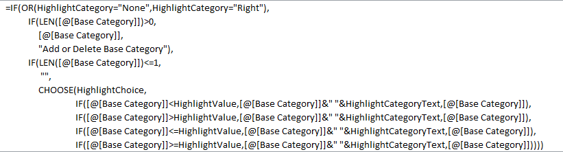
Notice that you can more clearly see the IF Function logical_test vs the [value_if_true] and [value_if_false] as well as the various values in the CHOOSE Function.

Consider using these Excel Formula Formatting techniques the next time you are writing complex calculations.

Video Demonstration

Check out this Video tutorial on the techniques presented above.

Would you use this technique?  Also, do you have any other Excel Formula Formatting tips and tricks?  Let me know in the comments below.

Steve=True