Create a Vertical Line Between Columns in Excel Using Error Bars
Thanks to Leonid (a super fan) for advising me on another and possibly better technique to create a vertical line between columns in your stacked column charts. This creates a visual separation on your charts. Thanks again, Leonid!
This technique uses Error bars to create the vertical line off of an XY Scatter chart. It helps to make sure that you don’t have to create the same data structure for a total and you can move it to the secondary axis to help fix the height. I think it looks great.
The Breakdown
1) Create a Stacked Column Chart
2) Create the XY Series Data
3) Add a New Series to the Chart
4) Move the Added Series to Secondary Axis and Change Added Series to XY Chart Type
5) Update the Added Series XY Values
6) Add Error Bars to the XY Chart Series and Format Error Bars
7) Change Secondary Vertical Axis Settings
8) Delete Legend Entry
Step-by-Step
1) Create a Stacked Column Chart
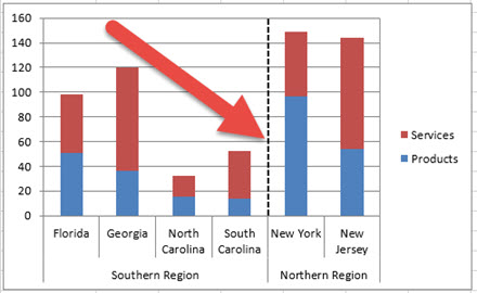
First, we need to create a stacked column chart type and this will help understand where the vertical line will be placed. If your chart data is set up in these cells and format:
| A | B | C | D | ||
|---|---|---|---|---|---|
| 1 | Products | Services | |||
| 2 | Southern Region | Florida | 51 | 47 | |
| 3 | Georgia | 36 | 84 | ||
| 4 | North Carolina | 15 | 17 | ||
| 5 | South Carolina | 14 | 38 | ||
| 6 | Northern Region | New York | 97 | 52 | |
| 7 | New Jersey | 54 | 90 |
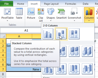
Then highlight the range A1:D7 and click on the Insert Ribbon and Select Stacked Column Chart:
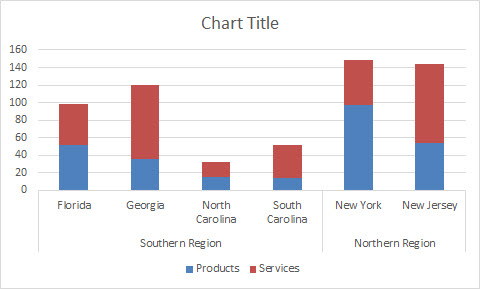
The chart will look like this in Excel 2016 (notice that the default is a Chart Title on Top of the Chart and the Legend at the bottom of the chart):
2) Create the XY Series Data
To make the vertical line, first, we must create data for an XY Scatter graph. So create a new chart data range for a vertical line. We want the vertical line between the 2 regions we have (i.e South Carolina & New York). Therefore, set up the following data in these cells as you see here:
| A | B | C | |
|---|---|---|---|
| 9 | Vertical Line | x | y |
| 10 | 4.5 | 0 | |
X Values:
We want the X value to be placed between the 4th & 5th columns. Excel sees each column with increments of 1. To put the vertical line between the regions of South Carolina and New York, we want a value of 4.5 for the XY series data point.
Y Values:
As we are not creating a line, and only a data point, we can leave this value as zero so that it starts at the bottom of the vertical axis, just at the horizontal axis.
3) Add a New Series to the Chart
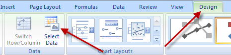
Next, we will add the new series to the graph that we will use Create a Vertical Line Between Columns. First click on the chart, then choose the Select Data button from the Design Ribbon.
Next, choose the Add button that you see in the Legend Entries (Series) area:
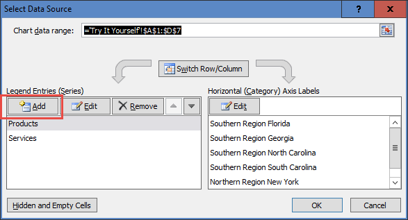
Then click on the following cells in the different cells and press okay to close on all dialog boxes:
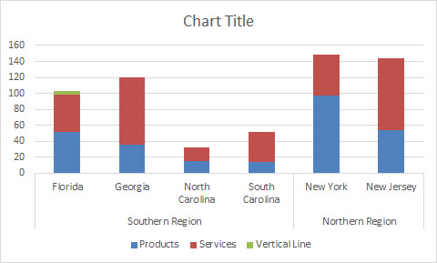
Now the chart will now look like this:
4) Move the Added Series to Secondary Axis and Change Added Series to XY Chart Type
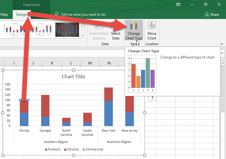
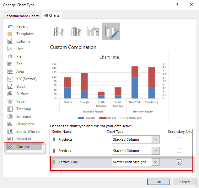
With the new series we just added, we need to change it to an XY Scatter Series and also to move it to the Secondary Axis. This is very easy in Excel 2016, so first, select your chart, and then select the Vertical Line Series and then click on the Change Chart Type Button on the Design Ribbon:
Then in the Change Chart Type dialog box under “Combo”, you should select “Scatter with Straight Line” in the Chart Type picklist and “Secondary Axis” checkbox next to the Vertical Line series as you see here:
Our chart now looks like this:

Notice that you do not see the XY Series as it is just a point on the horizontal axis. We will make it visible in the next steps.
5) Update the Added Series XY Values
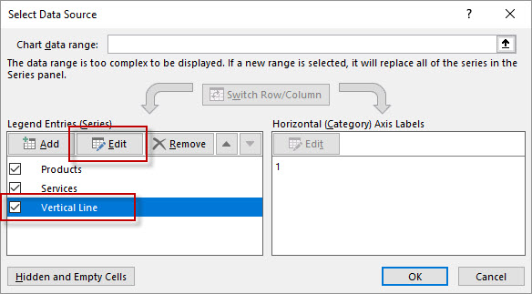
Now we should edit the XY Series so that it has both the x and y values. To do this, select the chart and then click on the Select Data button on the Design Ribbon:

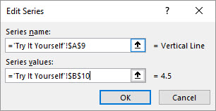
Click on the Vertical Line series and click on the Edit button in the Legend Entries (Series) area:
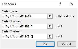
Next update the ranges of the X’s and Y’s to the ones you created in the previous step #2 as you see here:
Your chart should now look at this:
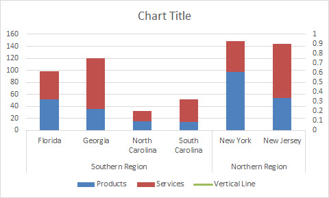
Note that it looks the same, but because we have set the Vertical Line as a data point with a Y = 0 the Secondary Vertical Axis has changed values. The line will show up in our next step from this point we just created.
6) Add Error Bars to XY Chart Series and Format Error Bars
Here is the where we create the vertical line. We will need to add an Error Bar to the Vertical Line Data Point. First, Select the Vertical Line Data Point located on the Horizontal Axis between the regions.
If you need help selecting the Vertical Line Series, check out this tutorial:
How-to Select Data Series in an Excel Chart when they are Un-selectable?
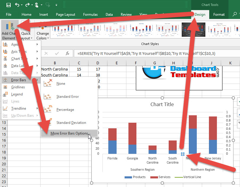
Once you have the Vertical Line Data Point selected, we need to add the error bars by going to the Design Ribbon and then choose the Add Chart Elements button and click on Error Bars and then More Error Bar Options…
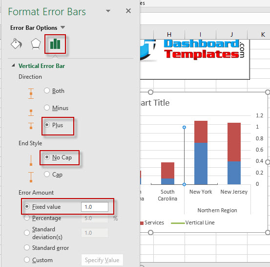
This will open the Format Error Bars for the Vertical Error Bars. Choose a Direction = Plus, and End Style = No Cap with a Fixed Error Amount of 1.0.
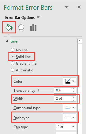
Next click on the Paint Can on the top of the dialog box to edit the Line Options and choose a Line=Solid Line, Color=Black, Width =2pt and Dash Type = Dash.
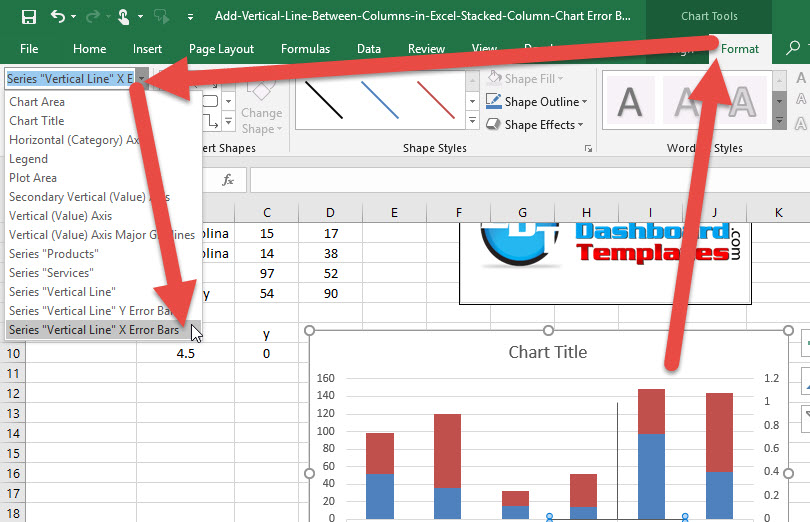
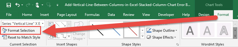
Next, select the Format Ribbon and change your Current Selection Picklist to Series “Vertical Line” X Error Bars:
Now click on the Format Selection button:
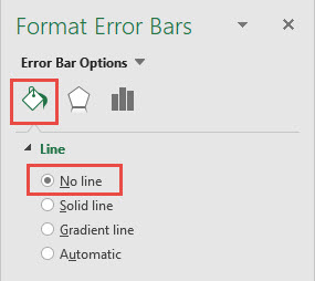
Finally, change the Horizontal Error Bars Line Options to “No Line”
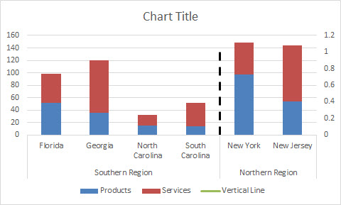
The chart with a Vertical Line Between Columns should now look like this:
8) Change Secondary Vertical Axis Settings
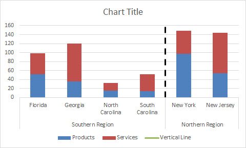
You can see that the Vertical Line is visible, but it doesn’t go high enough. So to make it look better, we need to change the Secondary Vertical Axis Settings by Double Clicking on it and then change the Minimum Bound = 0, Maximum Bound = 1, Tick Marks = None, and Labels = None.

Your chart should now look like this:
9) Delete the XY Series Legend Entry
Finally, just a little chart clean up to remove the extra legend entry for the Vertical Line series. First select the chart, then click on the legend. Then click on the Vertical Line Series legend entry and press the delete key. If you like you can also move the Legend to the right of your chart and the final chart looks like this:
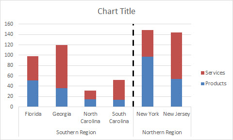
Understanding how to use Error Bars in Excel Charts is a great technique to know especially if you want to Create a Vertical Line Between Columns.
Video Demonstration
Check out this comprehensive Video on the Error Bar techniques presented above.
Sample File Download
Download the Completely Free Sample Excel Template File:
Create-Vertical-Line-Between-Columns-in-Excel-with-Error-Bars.xlsx
Do you use Error Bars in Charts? Let know your use case in the comments below.
Steve=True


