In this post, I will show you another Excel summation technique that you can use to evaluate criteria and then sum the data based on that criteria. Three posts ago, you received a challenge of summing 150,000 data points in many different ways. If you would like to try it out and then return to check your work, you can download the data here: Friday Challenge – Advanced Excel Summation Skills
Now as I showed you in previous videos, the fastest way is definitely a Pivot Table option. Here is a link to that post: Advanced Excel Summation Using A Pivot Table
Also, if you would like to check out a few other sum examples, check out this tutorial that uses SUMIFS as well as the SUMPRODUCT functions.
Array Formula Breakdown
An array is a collection of data items. Those data items can be in a single row or column (a one-dimensional array) or multiple rows and columns (a two-dimensional array). Three-dimensional arrays or array formulas are not available in Excel. An array formula can complete multiple calculations any number of items in an array that return either multiple resulting values or a single resulting value. NOTE: Array formulas require that you press CTRL+SHIFT+ENTER to make it calculate like an array in Excel.
For our formula, the array essentially holds all the values and then compares it against the criteria in a set of Nested If Statements within a Sum formula. It will then translate all of the data points vs the criteria into True’s and False’s. True data points will be considered in the final summation and False data points will not be added. In the simplest form of our Array Formula, lets consider all values by Store ID for only the first 8 data points. Here is a sample array formula that only checks for 1 criteria on just 8 rows.
In cell F47 enter this formula and then press CRTL+SHIFT+ENTER
=SUM(IF($B$2:$B$9=E47,$C$2:$C$9)) – You will then see the { } around the formula in the formula bar as you see here:
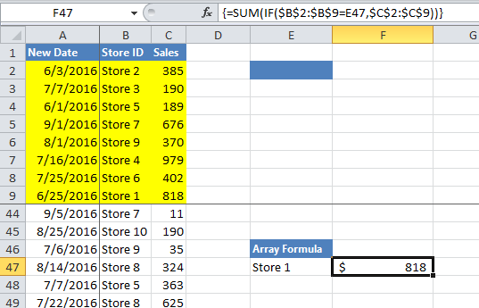
That is nice, but how does it work? To see what it is doing, highlight F47 and then go to the “Formulas” Ribbon and click on the “Evaluate Formulas” button in the Formula Auditing group.
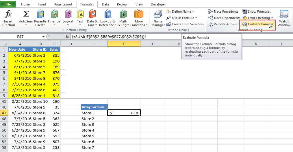
From there, you will then see this dialog box. Everytime you click on the evaluate button it will cycle through the math operations.
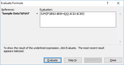
Sample Formula Breakdown
The formula is essentially going to evaluate the criteria in the IF function and then if it is true, it will return a range of sales data in cells C2:C9 to the Sum function. If it is not true, then only a False or Zero will be returned to the Sum Function.
Lets see it in action. Click on the “Evaluate” button and you will see this result in the dialog box:
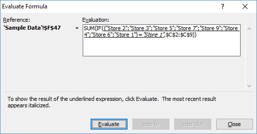
Notice that it has now filled in the store ids from the range B2:B9. It then compares that to our criteria in Cell E47 “Store 1”. Click on the Evaluate Button again in the dialog box to see the next step:
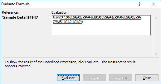
The formula evaluates the criteria against every value in the range and determines if it is True of False. Excel will funnel all of the True values to the Sum Function. So if the 1st, 3rd and 8th values were all true, then those resulting sales figures in the range C2:C9 would be submitted to the Sum formula. As you can see, only the 8th value is true, so only 1 value will be sent to the final Summation. Press the Evaluate button again and you will see what I mean:
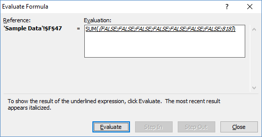
All the non-true values have a result of False and the 8th value was True so it shows the value of 818 in it’s place. Now Excel will either ignore the False values in the Sum Formula or translate them to Zero (0). Either way, the final sum value if the store ID = Store 1 for the range of sales data in cell C2:C9 = 818.
So now you have the basics, but lets update our formula for the multiple criteria that we need to check against given this data range for our data and formulas:
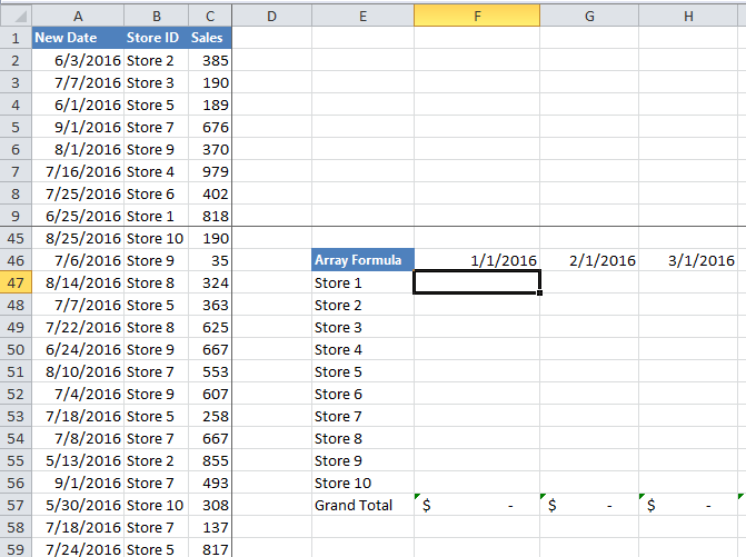
A2:A150,000 = Date Data
B2:B150,000 = Store ID Data
C2:C150,000 = Sales Data
Enter Array Formula in cell F47
E47:E56 = Store ID Summation Table Criteria
F46:R46 = Date Summation Table Criteria
Therefore, we will need to do the following for our Summation Calculation in 1 formula:
1) Sum the sales data by Store ID (Set as a value in the E column)
2) Sum the sales data by Month (Set as a value in the 46 numbered row)
Note to do this, we will need to create 2 criteria checkers. We can’t just check for the date in Cell F46 as that would only give us values for that exact date. So we will need to check and see if the sales data is greater than or equal to the date for the column the formula is in AND less than the adjacent column. It must be both and this will take 2 criteria checkers in our formula.
Here is the final formula that you can put in cell F47 but remember that you need to enter it with CTRL+SHIFT+ENTER to let Excel know to treat it as an Array formula.
=SUM(IF($B$2:$B$150000=$E47,IF($A$2:$A$150000>=F$46,IF($A$2:$A$150000<G$46,$C$2:$C$150000))))
Let’s break the formula down:
| Formula Steps | Description |
| =SUM( | We start with a SUM function as this is our evaluation of the final range of matching data. |
| IF($B$2:$B$150000=$E47, | First we need to check and see if the Store ID matches the Row 47 criteria |
| IF($A$2:$A$150000>=F$46, | Next we need to check and see if the Sales Date is >= Column F criteria (Current Column) |
| IF($A$2:$A$150000<G$46, | Next we need to check and see if the Sales Date is < Column G criteria (Adjacent Column) |
| $C$2:$C$150000)))) | Finally, return the Sales Data to the Summation formula and check it against the StoreID and Valid Date Range as above. |
If you have entered your formula correctly in cell F47, then you should get an answer of $337,425 for January 2016 for Store 1. If you are getting a Zero (0) value, then make sure you enter the formula with CTRL+SHIFT+ENTER to make it an Array formula. Make sure you check out the video below to help you understand each part of the Excel formula.
File Download
You can download the final file that includes all of the sample data and completed formulas so that you can see how they work here:
Friday-Challenge-Many-Sums-All-Sample-Formulas.xlsx
Video Demonstration
Please make sure you subscribe to my newsletter so that you get the next posting delivered directly to your inbox below.
Also, let me know in the comments below if there are any other formulas/functions that we could use so sum the sales data based on multiple criteria.
Steve=True


