This is part 1 of creating a dynamic Excel dashboard chart using the scroll bar control.
So in the title I said that we would be using a scroll bar to dynamically change the data in the Excel dashboard. For instance, I saw that a user had daily data for his organization and he wanted to show this data daily in the Excel dashboard chart and let the user select which day they wanted to see. So that is our use case. To show Excel dashboard chart data by day and let the user choose the day using a scroll bar.
BUT first, we need to know how to add a scroll bar to the Excel spreadsheet. Before you read on, take 5 minutes and see if you can find a way to add a scroll bar to your Excel spreadsheet.
Go on, look. Open up Excel and look for a way to do it.
Give up???
Okay, now that you tried on your own, lets see how I found it.
My first thought is that I am trying to INSERT something. In this case, a scroll bar.
So lets check out the INSERT Ribbon:
I don’t see anyway to insert a Scroll Bar, do you?
Then look at every other ribbon, and see if you see anything that says Scroll Bar. I don’t. ![]()
Why don’t we see it? It is because the default options in Excel are to HIDE the Developer Ribbon. Read on to see how you can add a Scroll Bar to your Excel spreadsheet.
How-to Add a Scroll Bar to your spreadsheet so that you can create a dynamic Excel dashboard:
In order to add a Scroll Bar to your spreadsheet for your Dynamic Dashboard creation, you first need to see the Insert Controls button. To see this, you need to add the Developer Ribbon or take at a little trick that I do. That trick is to add a Scroll Bar in your Excel worksheet is to Customize your “Quick Access Toolbar”.
The Quick Access Toolbar is the thing that you see at the top left of of your spreadsheet above above your Ribbons. This is where you see the Save icon, the Undo and Redo icons. You can add other tools that you frequently use and in this case the tools that you can’t find in any Ribbon. 
So you can add any command in this Quick Access Toolbar. I have a Insert Column Chart or Insert Line Chart as a standard command in my Quick Access Toolbar so that I can quickly create a chart of that type. You should look through all the choices so that you can add all the commands that you frequently use.
How-to Add a Command to the Quick Access Toolbar
So to add a command to your quick access toolbar, you need to select the down arrow next to the Undo command at the top left of your screen:
Then select the “More Commands…” menu option:
Now from the Choose Commands From: drop down list, choose Controls from the left menu and then press the “Add>>” button to move it to the right:
Then press the Okay button. Your Quick Access Toolbar will now look like this:

You will now see the Controls command appear in your Quick Access Toolbar.
To insert a scroll bar, you need to choose the Controls button from the Quick Access Toolbar and then choose the Insert button. Then choose the Scroll Bar control from the Form Controls section.
After you choose this control, you need to create the control in your spreadsheet by DRAG 
and DROP a range in the Excel worksheet:
You should now see this control in your spreadsheet.
Come back for the next installment of Part 2 of “How-to Create a Scroll Bar in Excel to Make Your Dashboard Dynamic” where we will create a chart that will use the scroll bar to let a user dynamically change the Excel dashboard chart.
Video Demonstration:
Here is a video tutorial on how to add a scroll bar to your Excel spreadsheet:
Also, don’t forget to subscribe to my blog and video channel so that you are sure to get the next installment delivered directly to your inbox. Also, my video subscribers receive discounts and promotions simply by being a subscriber. So do it already and subscribe! Also, let me know if you know of an easier way to add a scroll bar in a spreadsheet in the comments below.
Here is the sample data in case you want to try it out before I post my solution:
| A | B | C | D | |
|---|---|---|---|---|
| 1 | CT | Day | INC | AACD |
| 2 | 3PI_C | 3/1/2013 | 14 | 3 |
| 3 | 955CTS | 3/1/2013 | 2 | 1 |
| 4 | APPAU | 3/1/2013 | 12 | 8 |
| 5 | 3PI_C | 3/2/2013 | 9 | 0 |
| 6 | APPAU | 3/2/2013 | 39 | 17 |
| 7 | 3PI_C | 3/3/2013 | 11 | 15 |
| 8 | 955CTS | 3/3/2013 | 1 | 22 |
| 9 | APPAU | 3/3/2013 | 22 | 5 |
| 10 | APPAU | 3/4/2013 | 52 | 0 |
| 11 | 3PI_C | 3/5/2013 | 8 | 0 |
| 12 | 955CTS | 3/5/2013 | 2 | 9 |
| 13 | APPAU | 3/5/2013 | 39 | 17 |
| 14 | 3PI_C | 3/6/2013 | 44 | 27 |
| 15 | 955CTS | 3/6/2013 | 13 | 16 |
| 16 | APPAU | 3/6/2013 | 16 | 39 |
| 17 | 3PI_C | 3/7/2013 | 13 | 25 |
| 18 | APPAU | 3/7/2013 | 29 | 22 |
| 19 | 3PI_C | 3/8/2013 | 32 | 41 |
| 20 | 955CTS | 3/8/2013 | 10 | 5 |
| 21 | APPAU | 3/8/2013 | 15 | 18 |
Sheet2
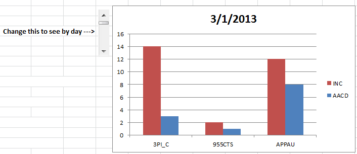
Here is what the first day will look like in the clustered column chart:
Update: You can view part 2 here:
how-to-make-a-dynamic-excel-scroll-bar-chart-part-2
Steve=True


