Welcome back to what I hope is the best site to learn all about tips and tricks to make your excel charts, excel graphs and excel dashboards.
When making your Excel Dashboards, you may be working with an EXTREMELY Large set of data. I frequently run into this, but if you do, you need to know how to navigate and select a large set of data without using very slow techniques. Now, I love my computer mouse, but I don’t usually use it when working with Excel and working with LARGE sets of data.
So, how large are your dashboard data sets?
Mine typically run into the 100,000 (100k) range. Therefore, you really need to know how to navigate such a large Excel Data Range.
First thing you need to do is learn how to select a large data range in Excel. This will save you time and ultimately save you money.
I was so frustrated when I used the mouse to select large data ranges. When you try and select a very very large data range, you will see that you may not do it easily because if you ever let go of your mouse, you selection will stop. Also, if your mouse or trackball is set to a very fast speed, you may find that i t is extremely difficult to select the Excel range.
So how can you select such large ranges for your formulas or copy and paste functions?
It can be really simple with Excel Keyboard Shortcuts, but if you do not know how to use these shortcuts, you will take you much longer to perform the same tasks and add much frustration to your task at hand.
The simple Excel Keyboard Shortcuts are:
CTRL + ARROW KEYS
or
CTRL + SHFT + ARROW KEYS
both of these shortcut keyboard key strokes will really save your day.
Lets examine both:
The first one is CTRL + ARROW KEYS.
This will allow you to quickly jump around your spreadsheet by moving your cursor to the next available Excel Cell of your next data range.
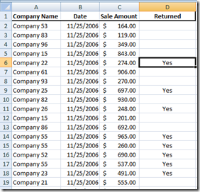
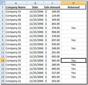
Here is how it works. Lets say that you have the following set of data and your active cell is D2 and wish to move as quickly as you can to the bottom of the data as you can near cell D18. Here is what you can do:
1) When your active cell is D2, 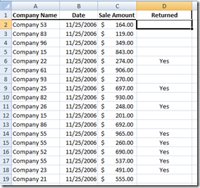 if you press and hold your control key (CTRL) down and then press your Down Arrow, you will immediately move your active cell to cell D6.
Then, if you keep the CTRL key depressed and keep pressing your Down Arrow, your active cell will jump to Cell D9, 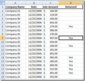
then if you keep doing it, your active cell will move to cell D11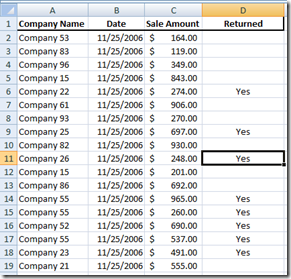
What is Excel doing? It is moving your to the next break in the data (if the next cell contains data) or the next cell that has data in it (if the next cell is blank).
Now you may be thinking that this is no big deal, but it is a BIG deal. What if the next break in the data is 34,000 rows away? It would take a long time to push the down arrow to row 34k or to click on the down scroll bar with your mouse. This is the speediest way. If the last row in your data is in row D34000, and you have no breaks from where you active selected cell of D2, then you will immediately jump down to D34000. It woks the same with the CTRL + Up Arrow or CTRL + Left Arrow or CTRL + Right Arrow. You will immediately jump to the next break in your data. Whether that is a the next data entry or the next space, you will move your active cell to that point. Please try this on your largest data set in all directions and then become very familiar with this as it will save you so much time using Excel.
Now, this is all fine and good to move to the next data break, but I wanted to HIGHLIGHT the data range, how do I do that?
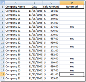
Basically, it is the same process as described above, but now you add the SHIFT key to the mix. Here are the same steps to highlight from cell D2 to D18. Starting from cell D2, press your CTRL+ SHIFT + DOWN Arrow to jump and highlight cells D2:D6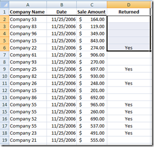
Then continue to hold down your SHIFT Key and CTRL key and then Press your Down Arrow again to highlight the range of D2:D9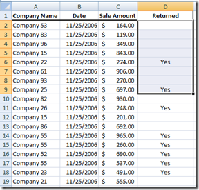
Continue to follow this process until you highlight the D2:D18 selection: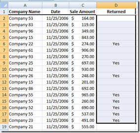
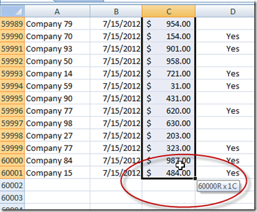
Once again, you may say how does this help me, but you will be able to SUPER DOOPER Quickly highlight a MASSIVE Data RANGE in only a few key strokes when you have very few breaks in your data:
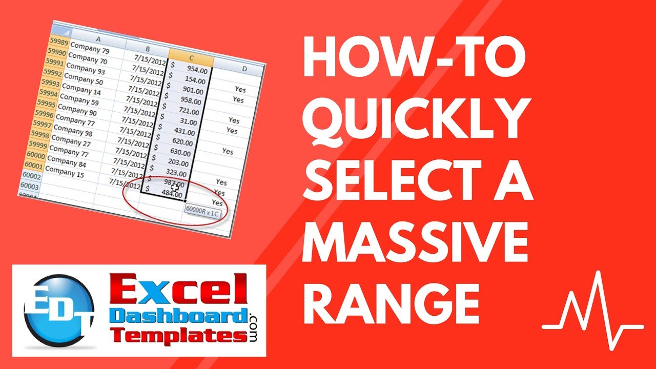
Look how I selected the data range from C2:C60000 because there was no breaks in the data.
This is another technique you MUST be comfortable with and be able to use at any time. This is an Excel Dashboard MUST technique.
Once you have mastered this incredibly AWESOME Excel technique, you just need to know one more twist, trick and tip to complete your Excel Jedi Training. What Excel tip and trick learn you must? It is the ability to move from CTRL + SHIFT with Arrows to just SHIFT + Arrows.
This will allow you to AWESOMELY Select a Massive data range in Excel and then just add or remove one more row or column. At any time you can add the CTRL or SHIFT keys back into the mix with your arrow keys to add or remove your range selection to Excel Spreadsheet.
When ever I have any selected range with the CTRL process, you can then release the CTRL key and while still selecting the SHIFT Key you can then press the Right or Left or Down or Up Arrows to change your selected Excel Data Range.e
Check out this video to see it ALL in action:
Also, don’t forget to sign up for my blog and my YouTube channel so you never, ever, ever, miss any Excel Dashboard Learning technique.
Let me know your latest Tip and Trick using Excel in the Comments below.
Steve=True

