Better late than never to the VLOOKUP week as started by Mr. Excel, Bill Jelen.
I have never been a big fan of the Excel VLOOKUP and even less a fan of the HLOOKUP functions in Excel. When I learned these functions in Excel, I had a few uses for them, but not too many. Also, I think I don’t like the HLOOKUP function because my brain always seems to put data with column headers with data in a vertical manner and not with row headers and data in a horizontal manner.
That being said, when I did learn the Vlookup formula, I think that the main reason problem I had with Vlookup was that I always seemed to have a large data set and I felt it was cumbersome to count the number of columns for the data that I wanted to return from the lookup function. It is a real pain in the butt. Also, what if my data changes and I need to lookup a value to the left of the Vlookup column? Vlookup will NOT allow you to put a MINUS in the Col_Index_Num. This means that you either have to copy the lookup value to the left of the data set. This can be a real problem with multiple data queries or if you are doing multiple VLookups.
So is there a better way to do a VLOOKUP without having to change your dataset? There is!!
Lets say your data looks like this: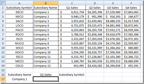
And lets say that you have the Subsidiary Name and you need to lookup the 1st Quarter Sales Revenue. That is easy for a Vlookup function and it would look like this: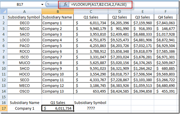
BUT what if all you wanted to return was the Subsidiary Symbol? You would have to copy the Subsidiary column to the right of the data set or copy/move the Subsidiary Name to the left of the Dataset. How can we make VLOOKUP go left?
Let’s us another formula for this Left VLOOKUP Function:
It uses a combination of Index and Match. This formula can really be tricky for some people, but it is such a great combination Excel formula that you can learn to use it just a quickly as VLookup and HLookup, and I would argue even faster than those Excel functions.
So how does it work?
First lets Learn more about the Index Function in Excel.
Here is what the Excel Help states on Index – Index Function “Returns a value or the reference to a value from within a table or range”. That sounds very similar to the Excel VLookup Function (“You can use the VLOOKUP function to search the first column of a range (range: Two or more cells on a sheet. The cells in a range can be adjacent or nonadjacent.) of cells, and then return a value from any cell on the same row of the range”)
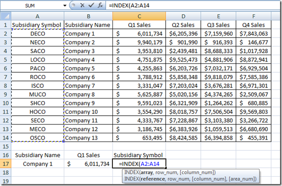
So we can return a value from an array using Index. Great! And that is what the first argument of the Excel Index Function. Excel wants to know what you want to return from an array. So in my example, I want to return the Subsidiary Symbol which is in Column A. So Lets put that in our function:
=INDEX(A2:A14
What this means is that Excel will return the Subsidiary Symbol as our final result and we always pick that out first. What do you want Excel to return?
Next we need to tell excel which row that the Subsidiary Name is in so that we can return the Subsidiary Symbol. Essentially, we need to match the Subsidiary Name in A17 to the list of names in Column B and then return that Row Number so that the Index formula can return the right symbol. Did you catch that?
We need to MATCH A17 with a value in Column B. So lets add that to the formula: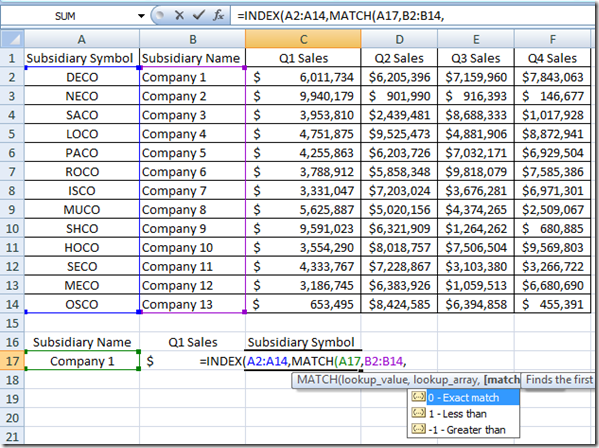
MATCH(A17,B2:B14,0)
Now we have selected that we want the Index Function to return the Subsidiary Symbol where it matches the same row as Company 1, the final step in the operation is to find out what column of data that we want to MATCH? Well in our example, we only provided one column of data in our Index array, so the answer to this always going to be 1 in this example.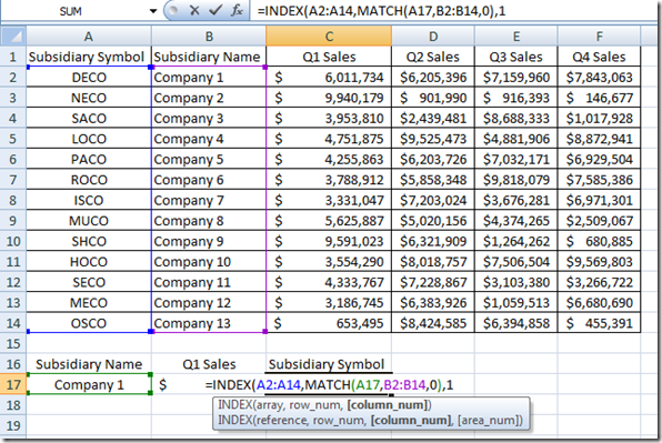
If you want, you can make your index function array really large and then match both the Column and Row, however, just using Index/Match in the way I describe above allows you to replicate a VLookup and also go left or right or even to another worksheet. There is no reason that your array/range has to be connected. The only requirement is that the count of your Matching rows equal the Index Array count.
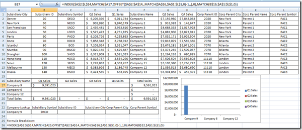
Here is a quick picture of how I have used a combination of Index and Match in a formula so that the lookup will dynamically find the column that contains Subsidiary Name and then use that as the matching column for the Index/Match lookup. Here is what that formula looks like and a picture of the data.
=INDEX($A$2:$L$14,MATCH($A17,OFFSET($A$2:$A$14,,MATCH($A$16,$A$1:$L$1,0)-1,,),0),MATCH(B$16,$A$1:$L$1,0))
But that is for another post as we need to breakdown each part of the formula.
So lets breakdown the Index/Match Function that we covered above
=INDEX(A2:A14,MATCH(A17,B2:B14,0),1)
=Index([Return What Value],Match([Match What Value],[To What Range],0),1)
Use INDEX/MATCH to create your lookup formula:
Here is the formula in simple terms:
=INDEX(
[Put in the Range of Data you want to Return],
MATCH([
Find what?],
[Find it Where?],
0 [for exact match])
1 [because you will only search in 1 column of data])
The reason you need to know this is that you can now use formulas like this to create your charts and graphs in your executive and company dashboards. We will use these formulas more extensively to make Dynamic Dashboards. I really hope this is helpful. I will try an post more detailed examples of this technique and most Excel designers need to understand this complex concept.
Please sign up for my blog in the RSS feed and also let me know what questions you have on this topic by leaving me a comment. Thanks!
Steve=True


