Okay, the client is always requesting changes. How do you deal with these? I suggest increasing the contracted hours. In this case, I decided to double the rate and double the billable hours. Since it was a free request, 2 x 0 (hourly Rate) x 10 billable hours = 0 ![]() (darn, I should have increased the hourly rate from zero, then doubling the hourly rate would have meant more.)
(darn, I should have increased the hourly rate from zero, then doubling the hourly rate would have meant more.)
Anyway, on to the problem and the solution.
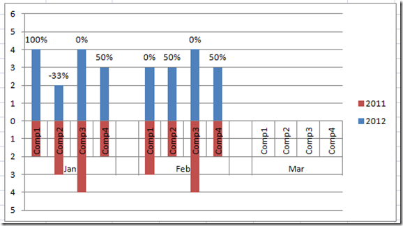
The client (code named GingerTrees) now wants a change to the original design that his/her boss sketched out on a napkin. GT (for short) now wants to put in a value of the percent change as a label on top of the upper columns.
Also, in this process, I realized we can simplify the creation of the chart. So lets take a look.
The Breakdown:
1) Create a Chart area with the previous year as a negative number.
2) Add 2 columns for the percent change from year to year (one positive and one negative)
3) Create a Stacked Column Chart
4) For Labels Series, add Labels.
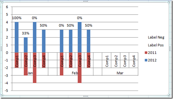
5) Change Fill of Both Labels Series = No Fill
6) Delete “Labels” from Legend
7) Remove “-“ sign from Vertical Axis Negative Values
8) Add a “-‘” Negative sign to the Label Values for Negative Labels.
Step-by-Step Instructions
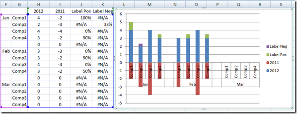
1) Create a Chart area with the previous year as a negative number.
H2 formula: =c2
I2 formula: =-d2 (negative d2)
Copy these formulas down. Don’t worry about the zeros as they will be ignored by the chart.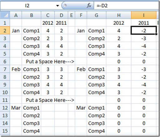
2) Add 2 columns. One for the percent change from year to year positive and one negative. Excel trick is to make the negative column the absolute value so that it shows a positive number and puts the label on top. Then we will change the display to make it look negative.
So that we don’t get a Divided by Zero Error (#DIV/0! Excel Error), put this formula in J2
J2: =IF(AND(ISNUMBER(D2),ISNUMBER(C2)),IF((C2-D2)/D2>=0,(C2-D2)/D2,NA()),NA())
K2: =IF(AND(ISNUMBER(D2),ISNUMBER(C2)),IF((C2-D2)/D2>=0,NA(),ABS((C2-D2)/D2)),NA())
The N/A will be ignored by the chart that we will create.
3) Create a Stacked Column Chart
Highlight the F1:K15 range and insert a 2D Stacked Column Chart.
4) Add labels for the label series.
Click on the Labels Series.
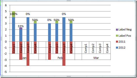
Click on the Layout Ribbon, Choose Data Labels and then Select Inside Base.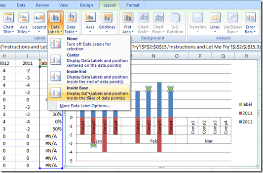
Your result will look like this:
5) Change Fill of Labels Series = No Fill
Right Click on the Label Series and select Format Data Series…
Then Select the Fill Submenu and then Choose No Fill.
6) Delete “Labels” from Legend
To do this in Excel, Select the ‘labels’ Legend item and press your delete key.
7) Remove “-“ sign from Vertical Axis Negative Values.
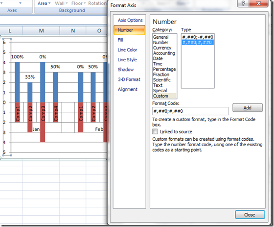
Right Click on the Chart Vertical Axis and choose Format Axis. Then choose the Number submenu, then put in this Format Code #,##0;#,##0 and press the Add button.
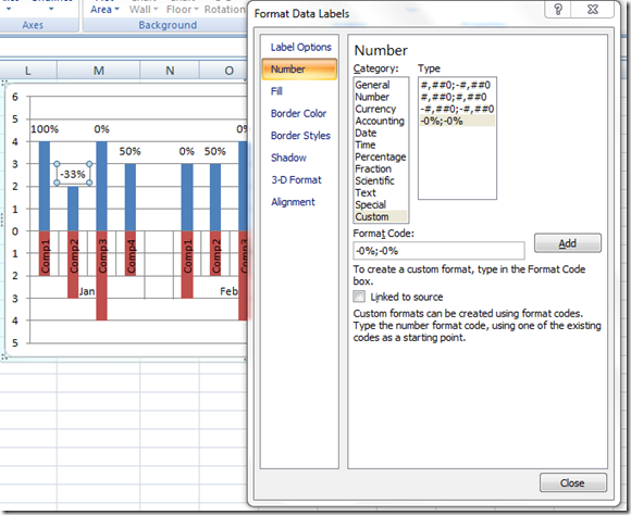
8) Right Click on the Labels that should be negative and select Format Labels. In our case it is the 2nd label of 33%. It should show –33%.
Then Click on the Number Submenu and put this in the Format Code:
-0%;-0%
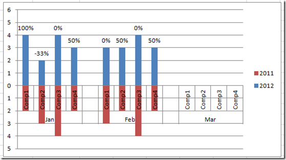
There you have it. Floating Labels for the percentage of change from one year to the next including negative numbers presented as a horizontal Tornado Chart in Excel.
Video Demonstration
Free Sample Download File
Excel-Horizontal-Tornado-Chart-Sample-File.xlsx
Please let me know if you found this helpful in the comments section below.
Also make sure you add your name to my mailing list so you get the next post in your inbox.
Thanks!
Steve=True

