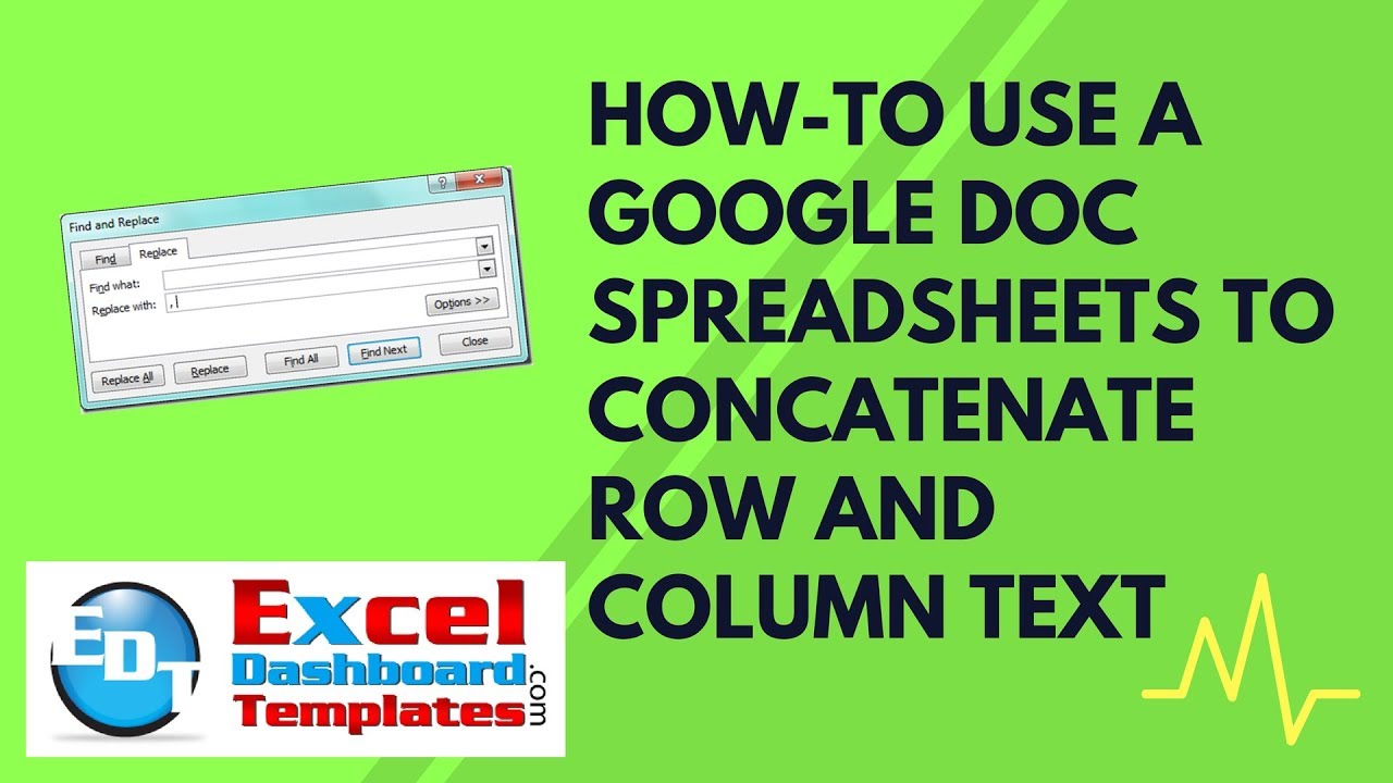
Yesterday I demonstrated how to find and replace a hard return in an Excel spreadsheet. I presented the last topic before this one so that we didn’t have to focus on that particular step. You can read about that Excel Tip & Trick post here:
How-to Find and Replace a Hard Return in an Excel Spreadsheet
Okay, now to the meat of this post. I was trying to Concatenate a series of values from different rows and put them into one cell. Essentially, I was trying to take the values in Column A1:A7 and put them in one cell (B1) separated by commas and a space. Like this:
In order to do this, I normally create a Concatenate formula in cell B1, like this:
=A1&”, “&A2&”, “&A3&”, “&A4&”, “&A5&”, “&A6&”, “&A7
Now if you want to know why I don’t have the word Concatenate anywhere in this formula, then you should check out this post:
How NOT to use Concatenate Function to build Dynamic Text in your Excel Dashboard Templates
Now writing this Concatenate formula is so long and a pain to make. So I wondered if there was an easier way to do this.
**If you know of a have a better formula that can concatenate and can scale with a highlighted range, please let me know. Maybe some sort of array formula? I don’t know and couldn’t find one or think of one. So let me know and I will write up a posting and video demonstrating it.
Now back to my story ![]() Okay, so for my company and most of the clients, we use a lot of Google Docs and Google Spreadsheets. And while working in both Excel and Google Docs, I found this awesome way to quickly concatenate a range of data in either rows or columns. Check it out.
Okay, so for my company and most of the clients, we use a lot of Google Docs and Google Spreadsheets. And while working in both Excel and Google Docs, I found this awesome way to quickly concatenate a range of data in either rows or columns. Check it out.
The Breakdown
1) Open up a Google Doc Spreadsheet
2) Highlight and Copy the Range of Data to Concatenate in Excel and Switch to Google Spreadsheet
3) Edit a Cell in Google Spreadsheet and Paste Information from Excel
4) Copy Newly Concatenated Cell and Switch to Excel
5) Edit a Cell in Excel Spreadsheet and Paste Information from Google
6) Find and Replace Hard Returns (If Copied from Rows) or Spaces (If Copied from Columns)
Step-by-Step
1) Open up a Google Doc Spreadsheet
Now you need access to Google Docs and you need to Create a Spreadsheet. 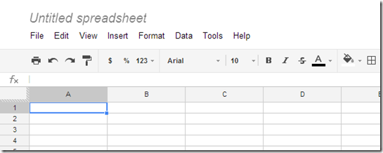
2) Highlight and Copy the Range of Data to Concatenate in Excel and Switch to Google Spreadsheet
Now that you have a Google Spreadsheet open, go back to Excel and Highlight your data range that you want to Concatenate into one cell.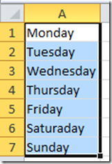
Once you have your range highlighted, press CTRL+C to copy the range. Now that you have the clipboard full of your data range, you need to switch back to the Google Spreadsheet.
3) Edit a Cell in Google Spreadsheet and Paste Information from Excel
Now that you are in the Google Spreadsheet, you need to Double-Click on any cell to get into the Edit mode of the cell: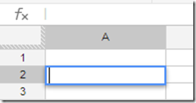
See how there is a curser in the cell, that means that we are editing the cell contents. Once you are at this point, press CTRL+V to paste the data within the cell in the Google Spreadsheet.
This is what the paste will look like: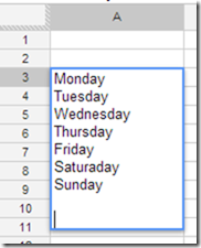
There may be a few extra hard returns that you can just press your backspace key until they are gone. When you finally press enter, you Google Doc will now look like this: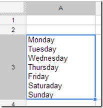
See how all of our data from many Excel Rows are now inside one cell in our Google Doc? I thought it was pretty neat. It also works for data in columns instead of rows. When you copy and paste data in columns, your pasted values will be separated by spaces and not hard returns. It would look like this:
4) Copy Newly Concatenated Cell and Switch to Excel
Now that you have your concatenation done in Google Spreadsheet, you can copy the cell from Google to Excel, but if you do this, you will notice that Excel will wrap the data in Double Quotes: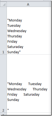
So I recommend actually editing the cell in the Google Spreadsheet so that you can get the data out with out having it wrapped in double quotes, like this: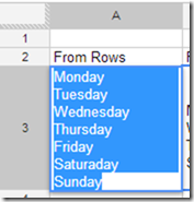
Now that you have edited and highlighted the concatenated data in the Google worksheet, press CTRL+C to copy the data. Then switch back to Excel.
5) Edit a Cell in Excel Spreadsheet and Paste Information from Google
Now when you are in Excel, you MUST Edit the cell that you want to put the concatenated data into and press CTRL+V to paste. Your resulting data will look like this: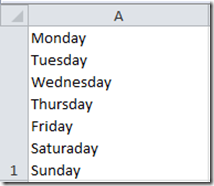
If you don’t follow this step, then your data will just be pasted back into the row format that you started with like this: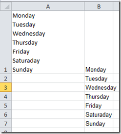
6) Find and Replace Hard Returns (If Copied from Rows) or Spaces (If Copied from Columns)
Once you are here, all you need to do is do a find and replace for the characters you don’t want with ones you do. If you are copying from rows, then check out this post:
How-to Find and Replace a Hard Return in an Excel Spreadsheet
If you are copying from columns, then I would recommend that you edit the cell and copy the exact number of spaces that is separating your data 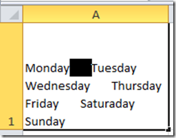 and put it into the find box:
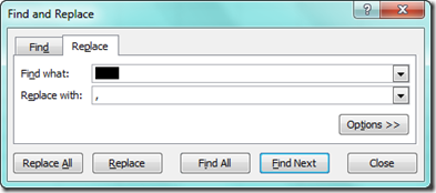
Once you finish your find and replace, your final data will look like this:
It is really very fast and should be faster than trying to create a concatenate formula for each and every cell. Especially for very large ranges. You can check out how fast and easy it is in this short video demonstration below.
Video Tutorial
If you have a formula can can do this faster and can work on any range, please let me know. Thanks
Steve=True


