In the recent Friday Challenge: Create Pipeline Usage Chart
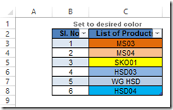
A user wanted to create a bar chart where the values had a specific color by product and also matched represented the size of the data.
Pete R. came up with an awesome VBA solution so that the colors will match the cell colors for a given product and apply those values to the bar chart.  Thanks Pete for the great solution.
Here is Pete’s write up:
I wanted to come up with a solution to the recent Friday Challenge, but I wanted the solution to be simple to implement, and dynamically updated. I thought that this challenge would be best solved with a little bit of VBA.
I started with a code that I found in “101 Ready-to-Use Excel Macros” written by Michael Alexander. This is listed in the book as Macro 83: Color Chart Series to Match Source Cell Colors. The code is as follows:
Private Sub MatchChartColors()
‘Step 1: Declare your variables
Dim oChart As Chart
Dim MySeries As Series
Dim FormulaSplit As Variant
Dim SourceRangeColor As Long
‘Step 2: Point to the active chart
On Error Resume Next
Set oChart = ActiveChart
‘Step 3: Exit if no chart has been selected
If oChart Is Nothing Then
MsgBox “You must select a chart first.”
Exit Sub
End If
‘Step 4: Loop through the chart series
For Each MySeries In oChart.SeriesCollection
‘Step 5: Get source data range for the target series
FormulaSplit = Split(MySeries.Formula, “,”)(2)
‘Step 6: Capture the color in the first cell
SourceRangeColor = Range(FormulaSplit).Item(1).Interior.Color
‘Step 7: Apply coloring
On Error Resume Next
MySeries.Format.Line.ForeColor.RGB = SourceRangeColor
MySeries.Format.Line.BackColor.RGB = SourceRangeColor
MySeries.Format.Fill.ForeColor.RGB = SourceRangeColor
If Not MySeries.MarkerStyle = xlMarkerStyleNone Then
MySeries.MarkerBackgroundColor = SourceRangeColor
MySeries.MarkerForegroundColor = SourceRangeColor
End If
‘Step 8: Move to the next series
Next MySeries
End Sub
The color matching macro worked great, but it did not dynamically change with new data entry. You would still have to manually color code all of the data to be charted and then run the macro to match the colors in the chart. I really wanted a method to perform some sort of LOOKUP of the data and return the colors. With that in mind I created the following bit of code:
Private Sub LookupColor()
Dim DataTable As Range
Dim DataCell As Range
Dim DataRangeColor As Long
Dim ColorTable As Range
Dim ColorCell As Range
Dim ValueRange As Range
Dim ValueCell As Range
Dim i As Integer
Dim Count As Long
Count = ThisWorkbook.ActiveSheet.Range(“E3”).Value
i = Count + 2
Set DataTable = Range(“D13: R13”) ‘ Adjust range as needed
Set ColorTable = Range(“C3: C” & i) ‘ Adjust range as needed
Set ValueRange = Range(“D14:R14”) ‘ Adjust range as needed
For Each ColorCell In ColorTable
For Each DataCell In DataTable
If DataCell.Value = ColorCell.Value Then
DataRangeColor = ColorCell.Interior.Color
DataCell.Interior.Color = DataRangeColor
End If
Next DataCell
Next ColorCell
For Each ValueCell In ValueRange
ValueCell.Interior.Color = ValueCell.Offset(-1, 0).Interior.Color
Next ValueCell
End Sub
This code defines the area of the sheet where the user defines the colors at the “ColorTable” and the individual cells that make it up as the “ColorCell”. The data range used to chart the data is defined as the “ValueRange” and each individual cell is a “ValueCell”.
There is a set of nested loops in the code. The code loops through each cell in the ColorTable and for each ColorCell loops through each DataCell in the DataTable and looks for a match in values. If the value in a DataCell matches a ColorCell then interior color (fill) of the DataCell will be made to match the ColorCell’s interior color (fill). Once the code loops through all of the DataCells it will move to the next ColorCell and continue looking for matches until all of the ColorCells have been run through the code.
Then I put all of the codes together and coordinate their actions in the correct order, I created the following code to drive it all:
Sub MatchColors()
Call LookupColor
Call MatchChartColors
End Sub
Finally to make it all simple to utilize I added a “Hot Key” (CTRL+SHIFT+M) to run the macro. I originally attempted to place button to control the macro, but since the code that matches the colors to the chart needed an active chart to be selected in order to operate, a button was not feasible. As soon as you click on the button it becomes the active object and not the chart, which cause the macro to fail. My solution was the “Hot Key” idea.
My final code is arranged like this:
Option Explicit
Sub MatchColors()
Call LookupColor
Call MatchChartColors
End Sub
Private Sub LookupColor()
Dim DataTable As Range
Dim DataCell As Range
Dim DataRangeColor As Long
Dim ColorTable As Range
Dim ColorCell As Range
Dim ValueRange As Range
Dim ValueCell As Range
Dim i As Integer
Dim Count As Long
Count = ThisWorkbook.ActiveSheet.Range(“E3”).Value
i = Count + 2
Set DataTable = Range(“D13: R13”) ‘ Adjust range as needed
Set ColorTable = Range(“C3: C” & i) ‘ Adjust range as needed
Set ValueRange = Range(“D14:R14”) ‘ Adjust range as needed
For Each ColorCell In ColorTable
For Each DataCell In DataTable
If DataCell.Value = ColorCell.Value Then
DataRangeColor = ColorCell.Interior.Color
DataCell.Interior.Color = DataRangeColor
End If
Next DataCell
Next ColorCell
For Each ValueCell In ValueRange
ValueCell.Interior.Color = ValueCell.Offset(-1, 0).Interior.Color
Next ValueCell
End Sub
Private Sub MatchChartColors()
‘Step 1: Declare your variables
Dim oChart As Chart
Dim MySeries As Series
Dim FormulaSplit As Variant
Dim SourceRangeColor As Long
‘Step 2: Point to the active chart
On Error Resume Next
Set oChart = ActiveChart
‘Step 3: Exit if no chart has been selected
If oChart Is Nothing Then
MsgBox “You must select a chart first.”
Exit Sub
End If
‘Step 4: Loop through the chart series
For Each MySeries In oChart.SeriesCollection
‘Step 5: Ger source data range for the target series
FormulaSplit = Split(MySeries.Formula, “,”)(2)
‘Step 6: Capture the color in the first cell
SourceRangeColor = Range(FormulaSplit).Item(1).Interior.Color
‘Step 7: Apply coloring
On Error Resume Next
MySeries.Format.Line.ForeColor.RGB = SourceRangeColor
MySeries.Format.Line.BackColor.RGB = SourceRangeColor
MySeries.Format.Fill.ForeColor.RGB = SourceRangeColor
If Not MySeries.MarkerStyle = xlMarkerStyleNone Then
MySeries.MarkerBackgroundColor = SourceRangeColor
MySeries.MarkerForegroundColor = SourceRangeColor
End If
‘Step 8: Move to the next series
Next MySeries
End Sub
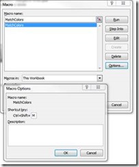
The last step I took was to assign a Shortcut key (Hot Key) to run the macro. To do this I opened the list of macros in This Workbook, selected the macro (MatchColors) and clicked Options. Then I set the Shortcut Key to CTRL+SHIFT+M.
Works like a charm. Thanks again for the great solution Pete!
Video Demonstration
Check out the video here:
File Download
Try the code by downloading the sample file here:
Friday Challenge Answer – Pipeline Usage Chart – Petes Answer – VBA Solution
Steve=True


