Wow, it has been over 2 years. I am so sorry if you have been waiting all this time. Probably not, but I will finish what I started with Part 2 of How-To Make a Dynamic Excel Scroll Bar Chart.
Here is a link to Part 1: how-to-create-a-scroll-bar-in-excel-to-make-your-dashboard-dynamic
The Breakdown
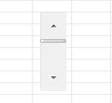
1) Insert a Scroll Bar Form Control
2) Create Calculations for Chart Series Offset Formulas
3) Update Scroll Bar Form Control Formats
4) Create Offset Named Formulas
5) Create Column Chart
6) Edit Chart Legend Entry (Series) and Horizontal (Category) Axis Labels
7) Insert Custom Chart Title
Step-by-Step
1) Insert a Scroll Bar Form Control
I have created a whole tutorial on this topic. Check out Part 1 to learn how to do this:
Part 1: how-to-create-a-scroll-bar-in-excel-to-make-your-dashboard-dynamic
After completing this, you will now have a scroll bar displayed on your worksheet.
2) Create Calculations for Chart Series Offset Formulas
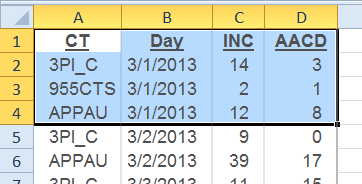
An Excel scroll bar will need an area to store the current selection/value. We will simply place a few data cells next to our original data set.
Here is the sample data for this tutorial:
| A | B | C | D | |
|---|---|---|---|---|
| 1 | CT | Day | INC | AACD |
| 2 | 3PI_C | 3/1/2013 | 14 | 3 |
| 3 | 955CTS | 3/1/2013 | 2 | 1 |
| 4 | APPAU | 3/1/2013 | 12 | 8 |
| 5 | 3PI_C | 3/2/2013 | 9 | 0 |
| 6 | APPAU | 3/2/2013 | 39 | 17 |
| 7 | 3PI_C | 3/3/2013 | 11 | 15 |
| 8 | 955CTS | 3/3/2013 | 1 | 22 |
| 9 | APPAU | 3/3/2013 | 22 | 5 |
| 10 | APPAU | 3/4/2013 | 52 | 0 |
| 11 | 3PI_C | 3/5/2013 | 8 | 0 |
| 12 | 955CTS | 3/5/2013 | 2 | 9 |
| 13 | APPAU | 3/5/2013 | 39 | 17 |
| 14 | 3PI_C | 3/6/2013 | 44 | 27 |
| 15 | 955CTS | 3/6/2013 | 13 | 16 |
| 16 | APPAU | 3/6/2013 | 16 | 39 |
| 17 | 3PI_C | 3/7/2013 | 13 | 25 |
| 18 | APPAU | 3/7/2013 | 29 | 22 |
| 19 | 3PI_C | 3/8/2013 | 32 | 41 |
| 20 | 955CTS | 3/8/2013 | 10 | 5 |
| 21 | APPAU | 3/8/2013 | 15 | 18 |
| F | G | |
|---|---|---|
| 3 | Minimum Date | 3/1/2013 |
| 4 | Scroll Value | 1 |
| 5 | Selected Date / Chart Title | 3/1/2013 |
| 6 | Date Row | 2 |
| 7 | Row Count | 3 |
Worksheet Formulas
|
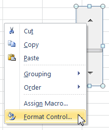
Now would be a good time to update our scroll bar formats.
To do this, right click on the Scroll Bar and click on the Format Control… menu item:
From there, you will then see a dialog box for the Scroll Bar. Change the values of the Scroll Bar as follows:
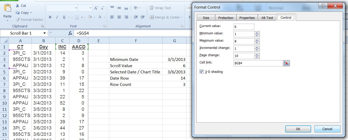
a) Current Value = Any Number between the Minimum Value and the Maximum Value
b) Minimum Value = I like to set it to 1 or 0. This will affect our formula for the Selected Date. If we put in 1, then we will need to subtract 1 from that formula. If we choose zero, then there is no need to subtract 1 from that formula.
c) Maximum Value = 7 or 8. This should be equal to number of dates that we have in our data set minus the minimum value we put in b) above.
d) Incremental Change =1 so that we move our dates on a day by day basis.
e) Page Change doesn’t matter in this case as we have a very small data set. If we had a larger data set, then page change affects how the scroll bar value increments when you click on the bar vs. the arrows.
4) Create Offset Named Formulas
For our Offset formula, we need to create 3 Defined Name formulas for the Chart Series Ranges and Horizontal Axis.
To do this, go to the Formulas Ribbon and Click on Define Name:
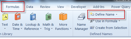
Then give your new Defined Name a Name and type in your offset formulas as follows:
ChartSeries1=OFFSET(‘Original Chart’!$A$1,’Original Chart’!$G$6-1,2,’Original Chart’!$G$7,1)
ChartSeries2=OFFSET(‘Original Chart’!$A$1,’Original Chart’!$G$6-1,3,’Original Chart’!$G$7,1)
ChartSeriesNames=OFFSET(‘Original Chart’!$A$1,’Original Chart’!$G$6-1,0,’Original Chart’!$G$7,1)
After you have created the chart series and axis Defined Name Formulas, we are ready to create our chart.
5) Create Column Chart
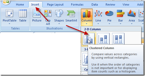
To create our dynamic chart, we want to first create a sample Column Chart that we will modify with our dynamic named formulas.
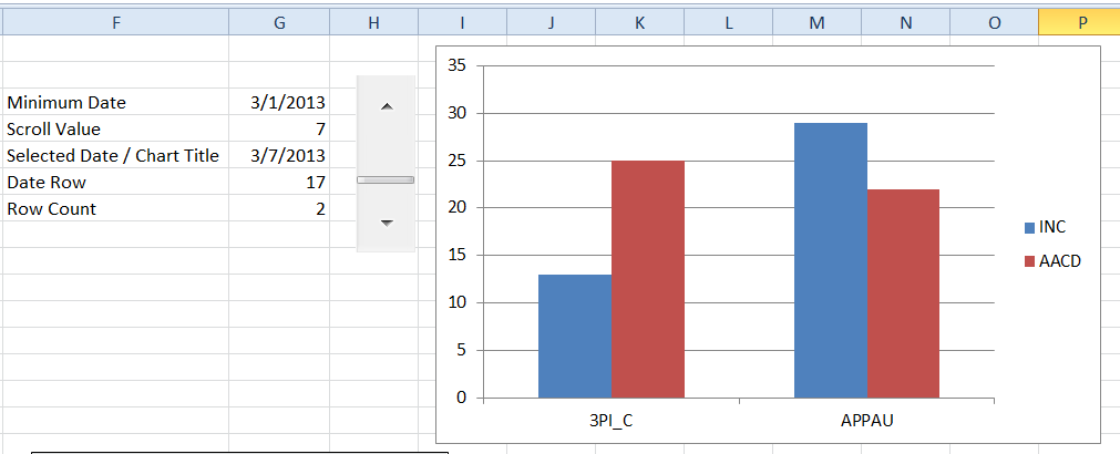
First, create a sample chart by highlighting the same data that would normally use to create a chart for 1 increment of the scroll bar. In this case, we will highlight 1 days worth of data as you see here:
Then Insert a 2-D Column Chart from the Insert Ribbon:
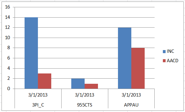
Your chart will now look like this:
6) Edit Chart Legend Entry (Series) and Horizontal (Category) Axis Labels
To edit our static chart series, first click on the chart, then click on the Design Ribbon and then on the Select Data button:
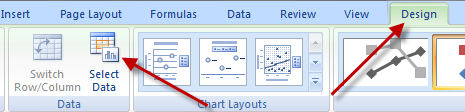
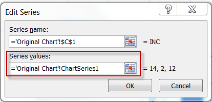
Then from the Select Data dialog box, click on the first series and then click on the Edit button on the Legend Entry (Series) area:
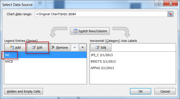
Change the Series Values to the Defined Name Offset Formula for ChartSeries1 you created above.
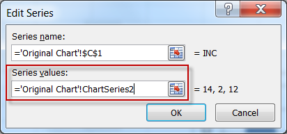
Repeat this step for ChartSeries2 you created above.
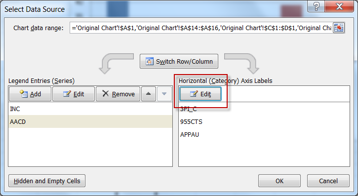
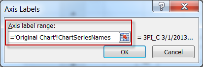
Then Change the Horizontal (Category) Axis Labels to the Defined Name Offset Formula for ChartSeriesNames you created above.
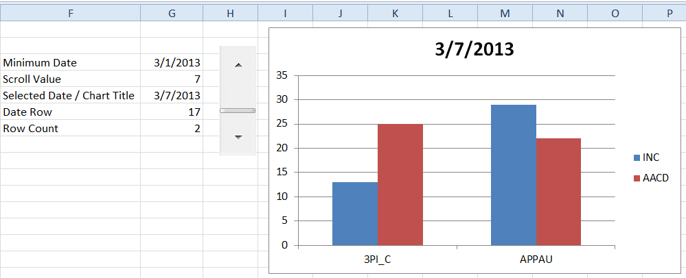
Your chart should now look like this when you scroll to March 7:
7) Insert Custom Chart Title
Finally, I feel that it is a good idea to tell the chart reader what data they have selected. I do this by changing the Chart Title to a dynamic link to a cell value. You may need to insert a Chart Title first from the Layout Ribbon. Then set the value of the Chart Title = $G$5
Here is a tutorial on this step:
Video Tutorial
Here is a demonstration of the Excel techniques shown above:
Sample File
Download the free sample Excel file here:
How-To-Make-a-Dynamic-Scroll-Bar-Chart-Part-2.xlsx
Thanks for the wait. What chart tutorials should we do next? Let us know in the comments below.
Steve=True


