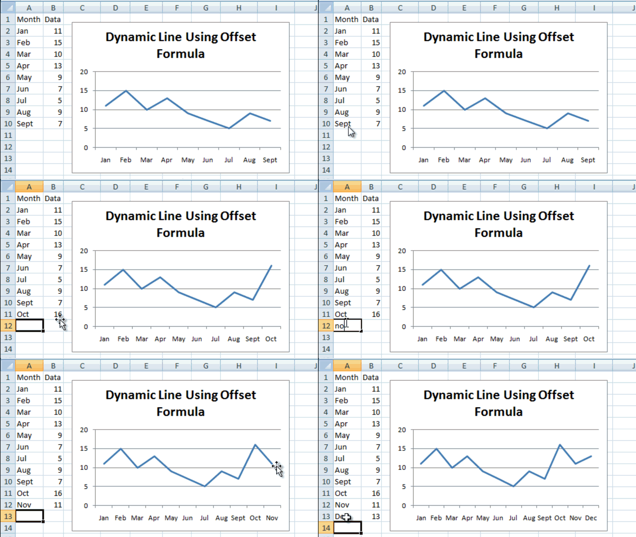
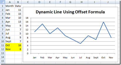
In previous posts I have described how to make a Dynamic Chart in Excel for your Dashboard using Tables. This is a very easy method to make a Dynamic Excel Graph, however, it may not have the flexibility that you desire. Perhaps your data cannot be easily put into a Table or perhaps the data is calculated in many different areas that are updated by users or perhaps you are using an older version of Excel like Excel 2003 and tables aren’t your friend. Also, it is perfect for almost any Dynamic Dashboard Template using Microsoft Excel. So how can we add more flexibility to our dynamic chart?
The Offset Function to the Rescue!!
Another great way to make a Dynamic Charts and Graphs is to use the Offset formula to create a dynamic range. I described how to use the Offset Function in this previous post: This is the Bomb: or How I came to love the Offset function. In essence, we are going to use the Offset function to define a range that can move and grow as users add more data. Every time a user puts in more data, the offset function can be used to find the beginning and end of the range and we can send that to the chart so that the most current data points are added to the graph.
The Breakdown
1) Define Named Ranges using the Offset Function that uses dynamic techniques for each data series and the X axis categories.
2) Create a chart adding the Named Ranges as the series and axis.
Very Important – This step MUST be done to the chart series not the chart data range as excel will translate the Offset named range to an actual range that will not remain dynamic.
Just as Important – When adding the named range to the chart series, you MUST reference both the file name as well as the named range…i.e. FileName!NamedRange.
Step-by-Step
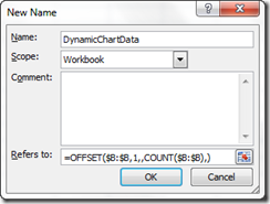
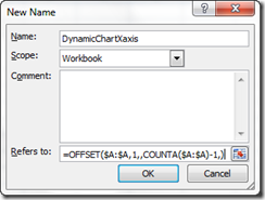
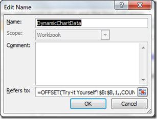
1) Create Name Ranges
DynamicChartData
=OFFSET($B:$B,1,,COUNT($B:$B),) DynamicChartXaxis=OFFSET($A:$A,1,,COUNTA($A:$A)-1,)
2) Create a New BLANK Chart in any cell below (not adjacent to the data so that you don’t have to delete anything and save some time)
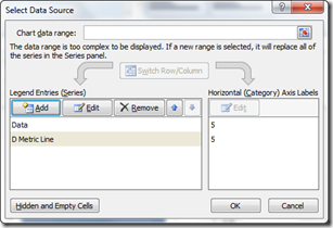
3) Select the Chart and then choose the Select Data Button in the Design Ribbon
4) Then Add – Legend Entry (Series)
=DynamicChartUsingOffsetDownload.xlsx!DynamicChartData
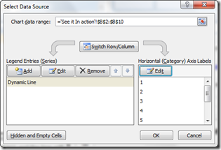
5) Select the Chart and then choose the Select Data Button in the Design Ribbon as in Step 3
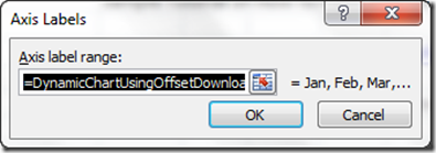
6) Then Change Horizontal Category (Xaxis)
=DynamicChartUsingOffsetDownload.xlsx!DynamicChartXAxis
7) Add new Data to Label and Data Columns (Column A and B) and watch the chart dynamically change!
Video Tutorial
Free Sample Download File
Dynamic-Chart-Tutorial-Using-Excel-Offset-Function.xlsx
Please let me know if you found this helpful by leaving me a comment and also sign up for my RSS Feed so you are sure to get the latest Excel Dashboard Tutorial.
Steve=True

